| motiv | harm | stabi | ppsych | ses | verbal | read | arith | spell | |
|---|---|---|---|---|---|---|---|---|---|
| 0 | -7.907122 | -5.075312 | -3.138836 | -17.800210 | 4.766450 | -3.633360 | -3.488981 | -9.989121 | -6.567873 |
| 1 | 1.751478 | -4.155847 | 3.520752 | 7.009367 | -6.048681 | -7.693461 | -4.520552 | 8.196238 | 8.778973 |
| 2 | 14.472570 | -4.540677 | 4.070600 | 23.734260 | -16.970670 | -3.909941 | -4.818170 | 7.529984 | -5.688716 |
| 3 | -1.165421 | -5.668406 | 2.600437 | 1.493158 | 1.396363 | 21.409450 | -3.138441 | 5.730547 | -2.915676 |
| 4 | -4.222899 | -10.072150 | -6.030737 | -5.985864 | -18.376400 | -1.438816 | -2.009742 | -0.623953 | -1.024624 |
Structural Causal Models in PyMC
Conditionalisation Strategies and Valid Causal Inference
2025-05-13
Preliminaries
Who am I?
- I’m a data scientist at Personio
- Bayesian statistician,
- Reformed philosopher and logician.
- Website: https://nathanielf.github.io/
Code or it didn’t Happen
- The worked examples used here can be found here
- Download SEM Notebook
- SEM Data

My Website
Form and Content of Causal Inference
Directed Acyclic Graphs and their Meaning
“Every proposition has a content and a form. We get the picture of the pure form if we abstract from the meaning of the single words, or symbols (so far as they have independent meanings)… By syntax in this general sense of the word I mean the rules which tell us in which connections only a word [makes] sense, thus excluding nonsensical structures.” - Wittgenstein Some Remarks on Logical Form
 \[ \psi | \neg \psi | \psi \rightarrow \phi \]
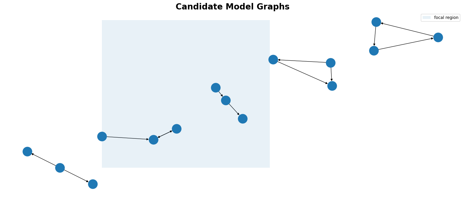
Sets of Admissable Graphs and Well formed valid Fomulae
Abstract Conception
Non-Parametric Structural Diagrams
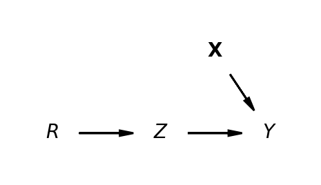
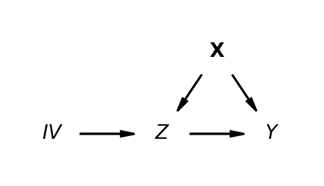
Non-parametric Structural Causal Models highlight the aspects of the Data Generating processes that threaten the valid construction of a causal claim.
\[ Y \sim f_{Y}(Z, X, U_{Y}) \] \[ Z \sim f_{Z}(X, IV, U_{Z})\] \[ X \sim f_{X}(U_{X})\] \[ IV \sim f_{IV}(U_{IV})\]
Concrete Conception
Parametric Approximation via Regression
\[ y \sim 1 + Z + u \] Regression Approximation to estimating valid coefficients in systems of simultaneous equation via 2SLS.
\[ y \sim 1 + \widehat{Z} + u \] \[ \widehat{Z} \sim 1 + IV + u \]
Functional Form and the State of the World
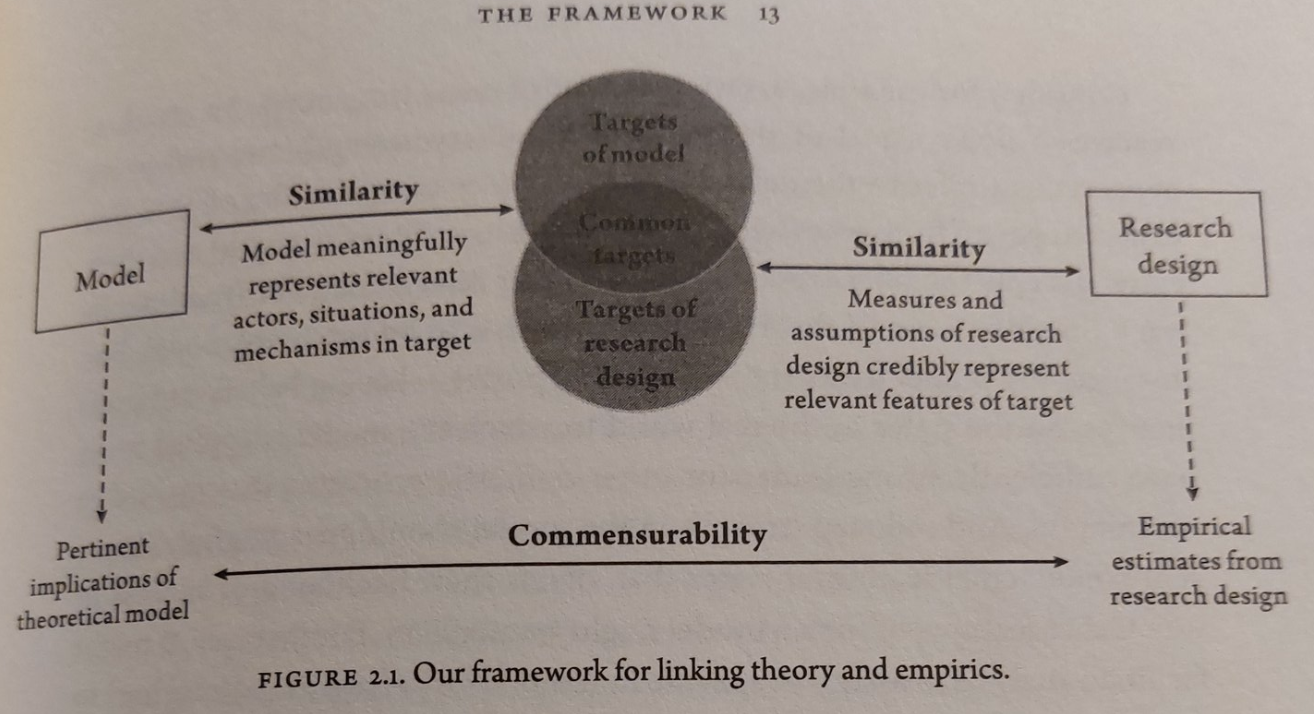
Credible Maps
Causal Structural Models generate valid causal claims just when:
- the mathematical model is apt to account for risks of confounding in the assumed data generating process
- the model parameters or theoretical estimands can be properly identified and estimated with the data available.
- the assumed data generating process is a close enough approximation of the actual process
- The set of admissable causal claims is constrained by the substantive extra-statistical requirement to credibly map model to the world
\[ \Bigg( \begin{array}{cc} Y \sim f_{Y}(Z, X, U_{Y}) \\ Z \sim f_{Z}(X, IV, U_{Z}) \end{array} \Bigg) \approxeq \Bigg[ \begin{array}{cc} Y \sim 1 + \widehat{Z} + u \\ \widehat{Z} \sim 1 + IV + u \end{array} \Bigg] \\ \approxeq \dfrac{p( (y_{1}, z_{1})^{T} ....(y_{q}, z_{q})^{T}) | \color{purple}\Sigma ,\color{blue}\beta \color{black} )p(\color{purple}\Sigma ,\color{blue}\beta \color{black}) }{\sum p_{i}(YZ)} \]
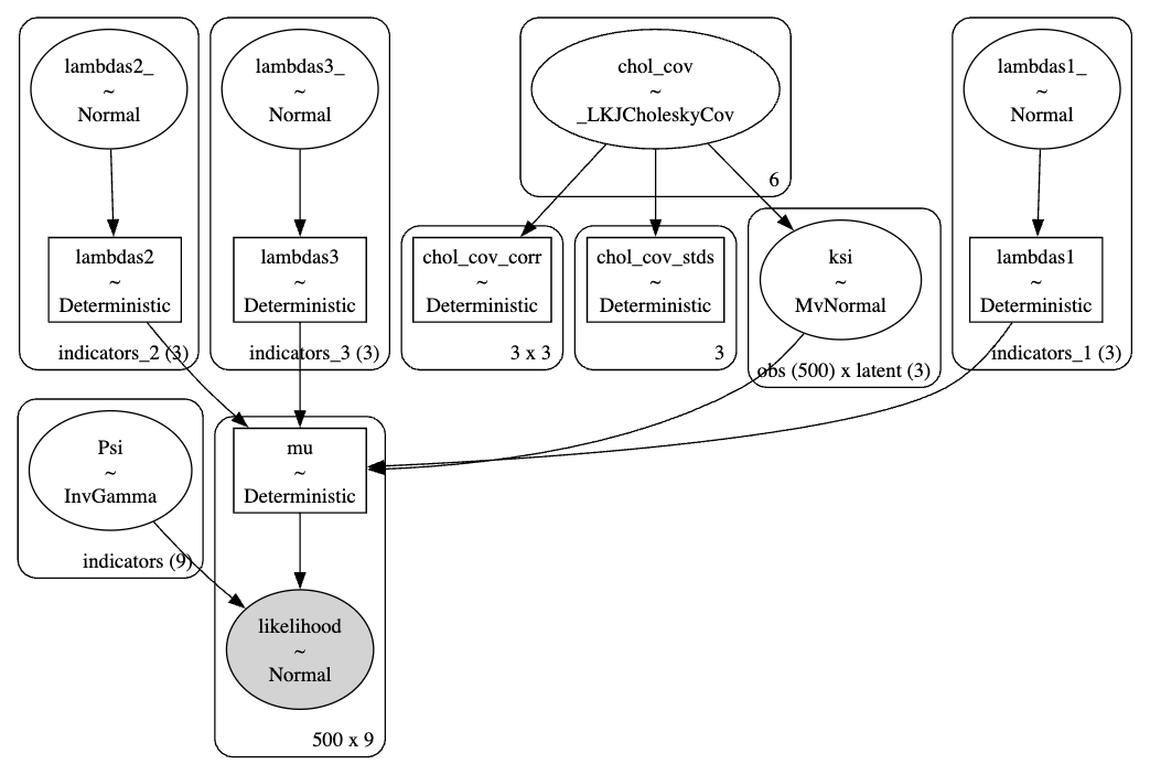
Factor Structures as Measurement Models
\[ ADJUST \sim f_{ADJUST}(motiv, harm, stabi, U) \] \[ RISK \sim f_{RISK}(ppsych, ses, verbal, U)\] \[ ACHIEVE \sim f_{ACHIEVE}(read, arith, spell, U)\]
Non-parametric phrasing of SCMs under-specifies the relations of interest.
CFA models estimates the multivariate correlation structure while imposing the focal causal structure and dependencies to “hide” detail in measurement error.
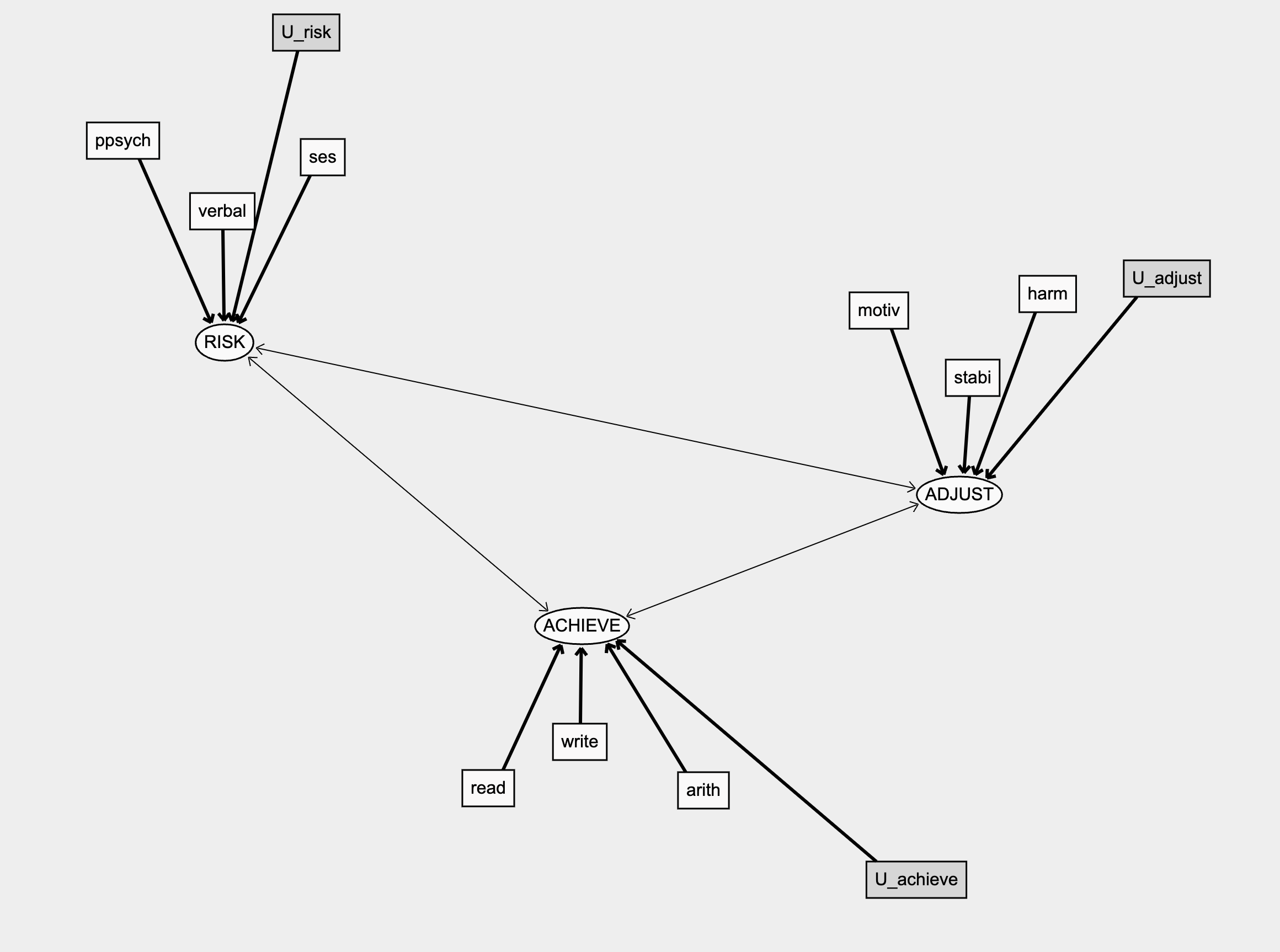
Measurement Model Graph
Model Estimates: Factor Loadings
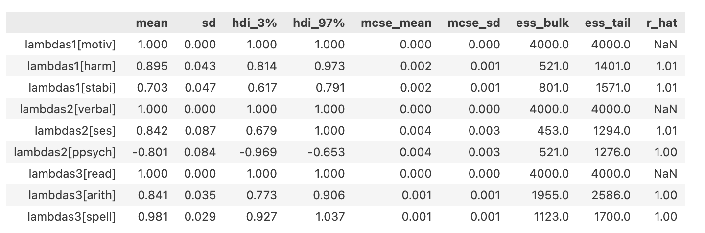
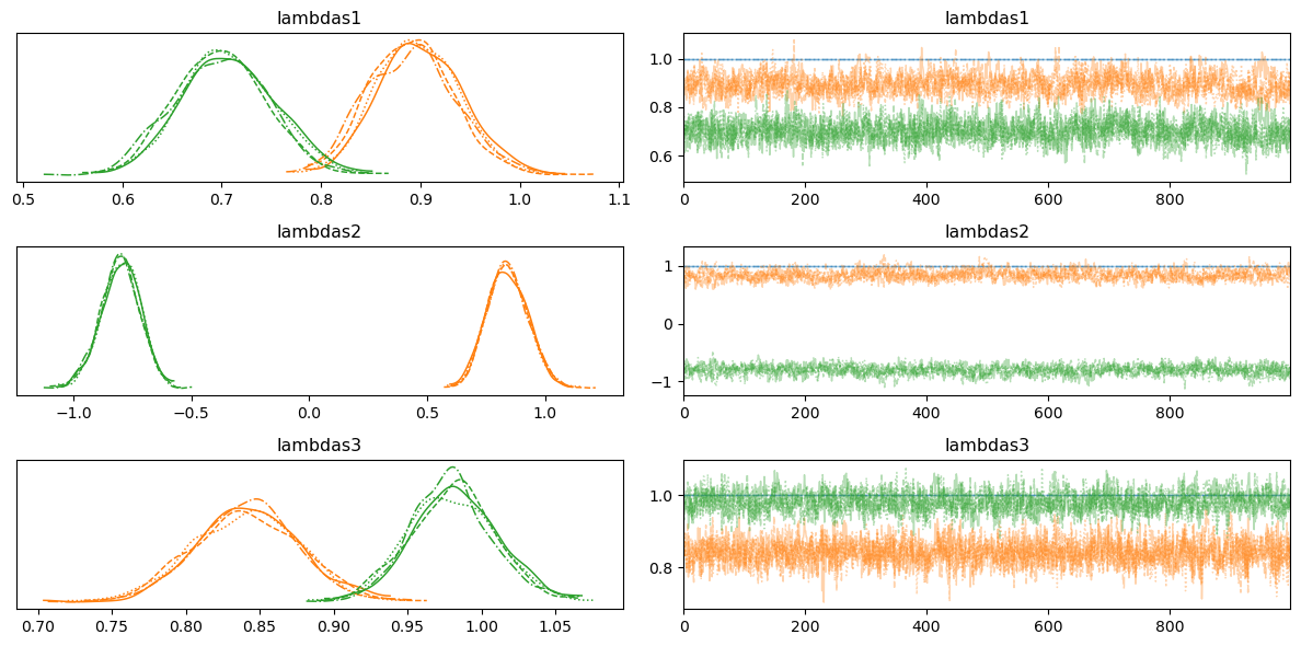
- The weights accorded to each of the indicator metrics on each of the specified factors are scaled.
- Consistency in the factor loadings is a gauge of factor coherence.
- Invariance of the loading scale across groups supports the argument to robust constructs.
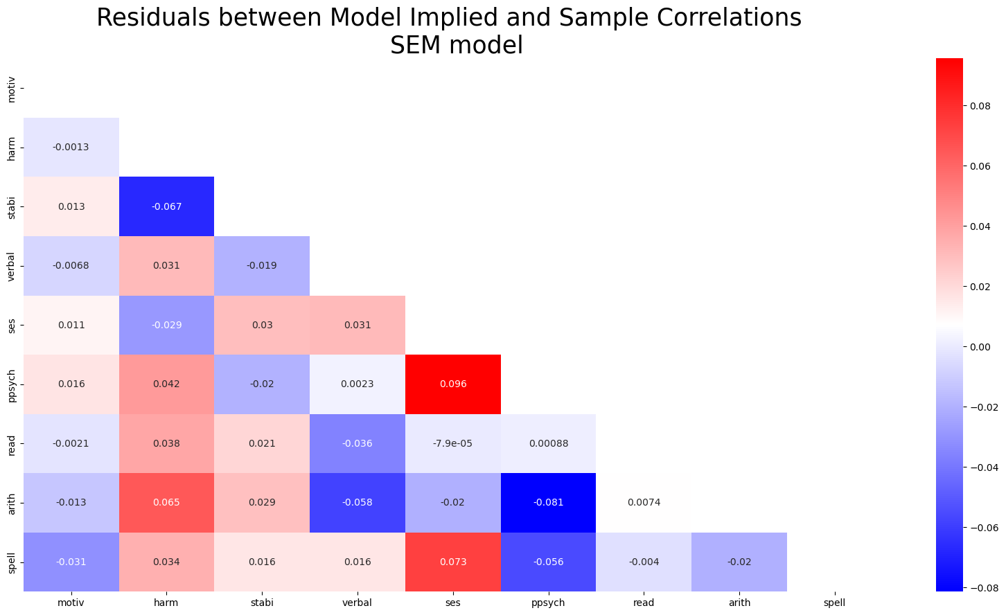
Model Fit: Covariance Structures
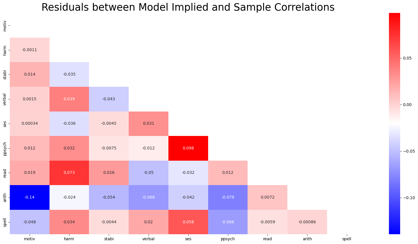 The differences between the sample covariance and model predicted covariances are small.
Model Fit: Posterior Predictive Checks
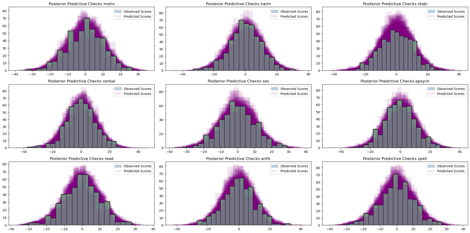 The model can successfully retrodict the observed data, indicating good model fit.
Model Implications: Latent Scores
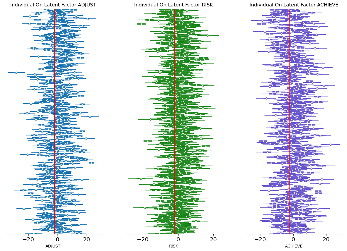
- Bayesian Models sample the Latent constructs
- Assess the measurement profile of individual outliers under intervention.
- Allows us to interrogate what are the relations between these Latent components?
- How do thet vary under pressure?
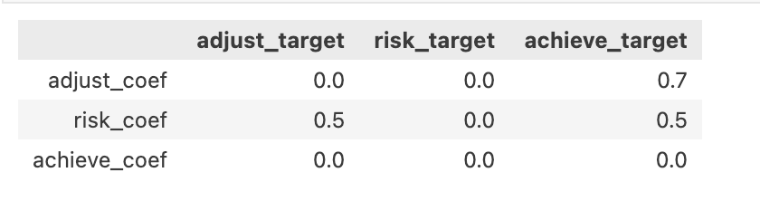
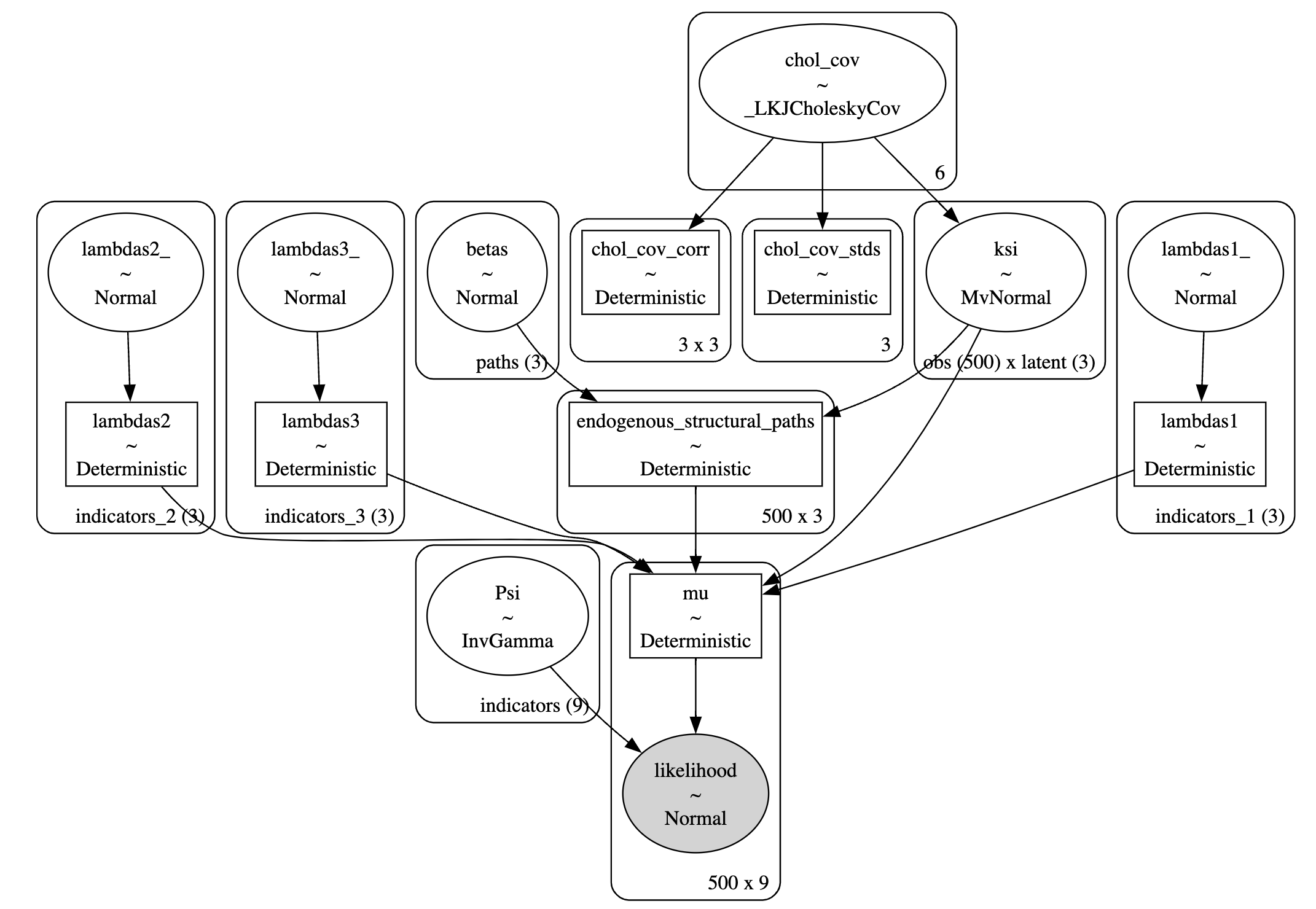
The Structural Matrix
\[ \overbrace{\text{Ksi}}^{latent} = \begin{bmatrix} \overbrace{2.5}^{adjust} & \overbrace{3.2}^{risk} & \overbrace{7.3}^{achieve} \\ ... & ... & ... \\ ... & ... & ... \\ ... & ... \\ 3.9 & ...\end{bmatrix} \begin{bmatrix} 0 & \beta_{12} & \beta_{13} \\ \beta_{21} & 0 & \beta_{23} \\ \beta_{31} & \beta_{32} & 0 \end{bmatrix} = \underbrace{\mathbf{B}}_{Regression \\ Coefficients} \]
Model Comparison
Local and Global Fit
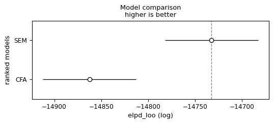
SEM model achieves better performance on the local and global model checks than the CFA model
Causal Estimands and the Do-Operator
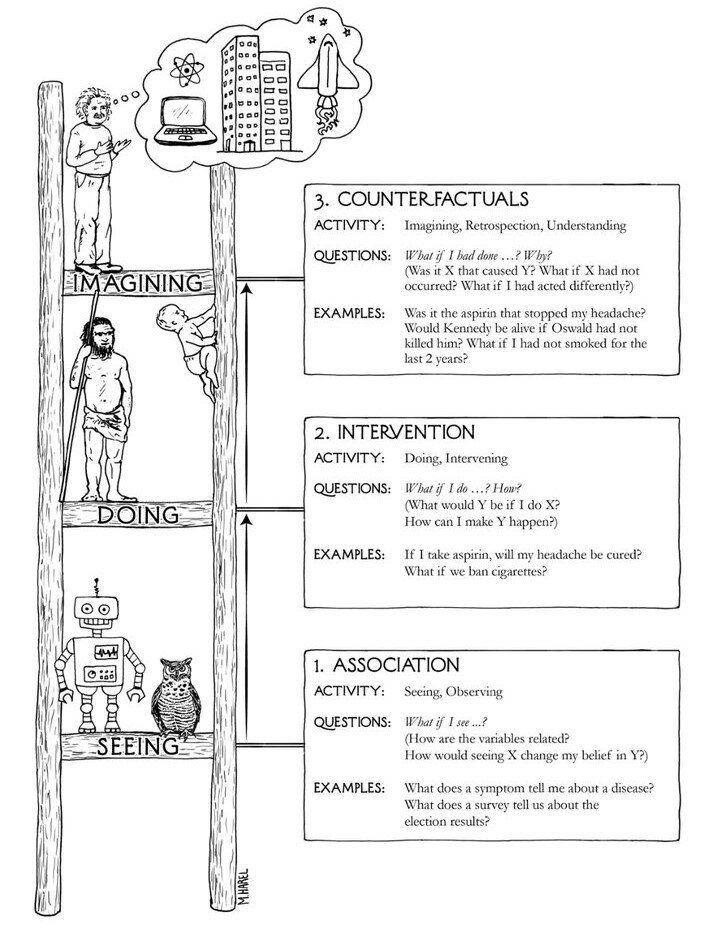
The graph algebra of the do-calculus sets rules on admissable structures required to warrant valid causal claims when accounting for different species of confounding.
They complement the development and analysis of SEM models, providing minimalist admissablility conditions for a causal interpretation of these structural relations.
The substantive justification of the causal claims implicit in a SEM model need to be made more explicitly by the researcher with reference to evaluation of model fit to data by comparing to competing models.
What-if Structures and the Do-Operator
“[T]ypically the causal assumptions are less established, though they should be defensible and consistent with the current state of knowledge. The analysis is done under the speculation of “what if these causal assumptions were true.” These latter analyses are useful because there are often ways of testing the model, or parts of it. These tests can be helpful in rejecting one or more of the causal assumptions, thereby revealing flaws in specification. Of course, passing these tests does not prove the validity of the causal assumptions, but it lends credibility to them.”
- Bollen and Pearl in Eight myths about causality and structural equation models
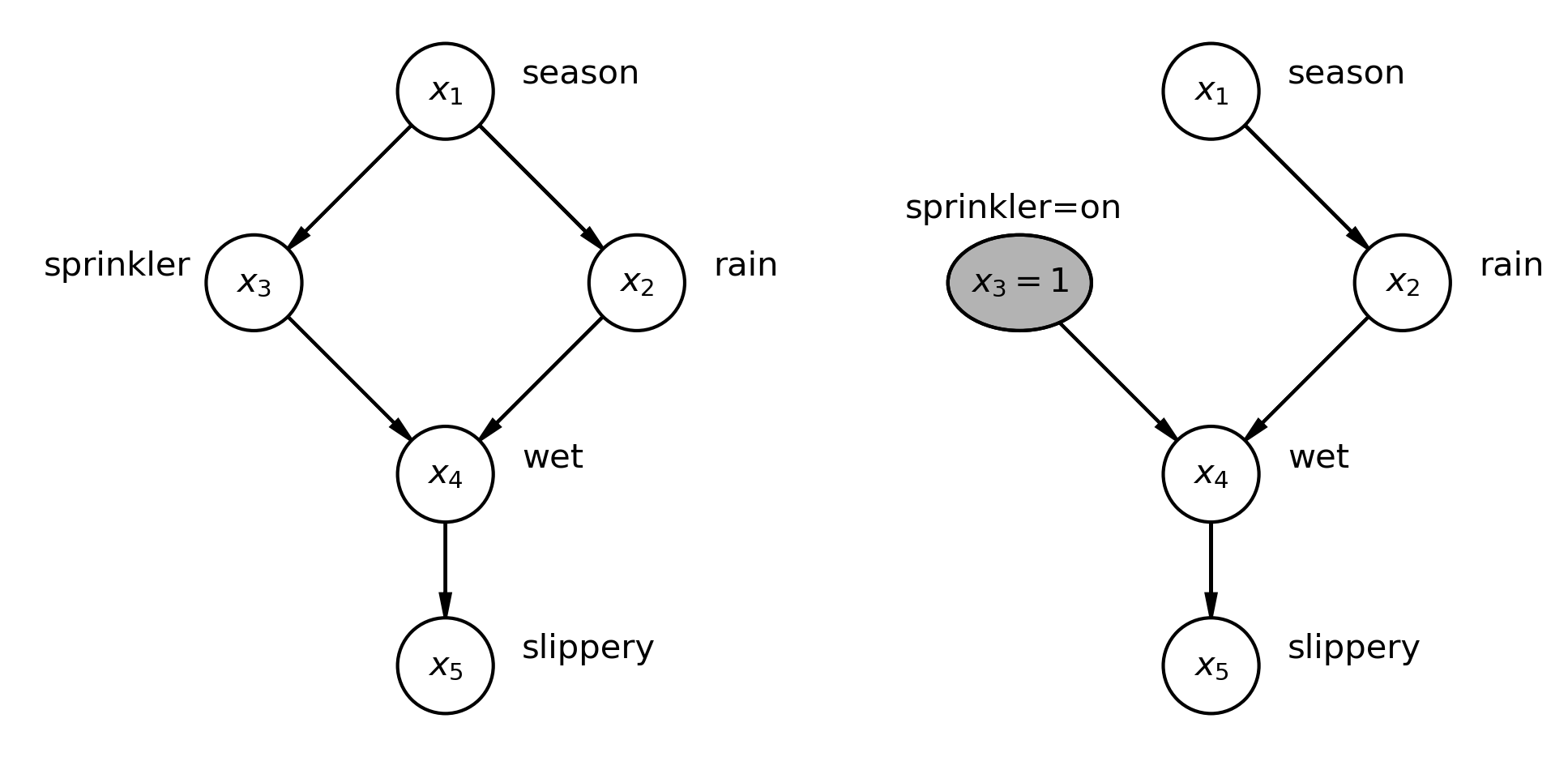
The Do-Operator uses graph mutilation techniques to interrogate the impact of different data generating conditions including the analysis of causal claims.
Graph Mutilation in PyMC
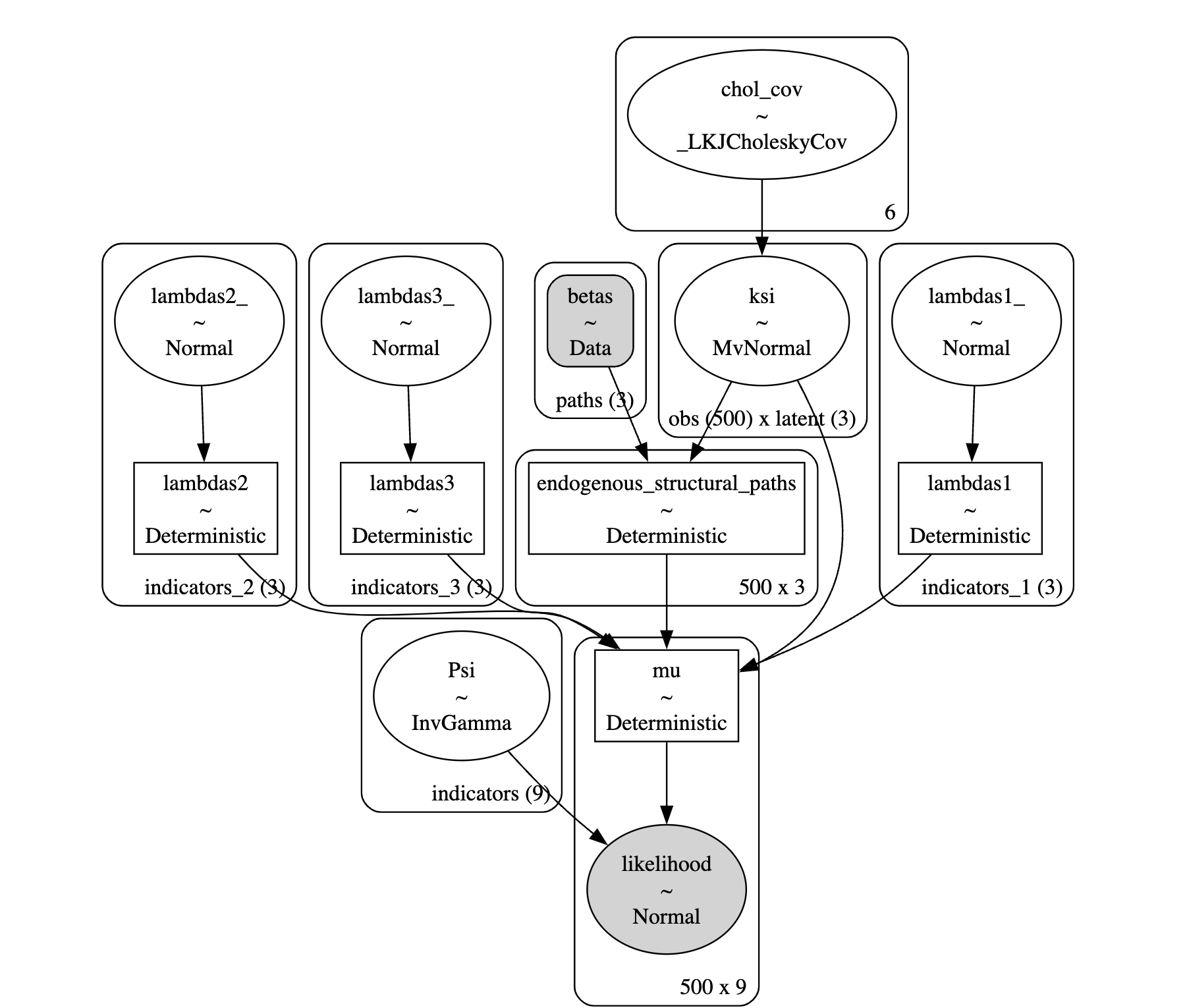
Causal Estimands under Intervention
\[ E\Big[(Y| do(\beta=0)) - (Y | do(\beta \neq 0) \Big] \] 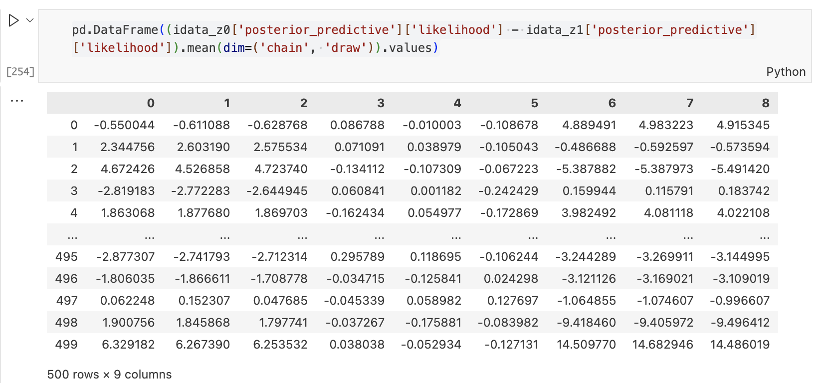
Model Fit: Sensitivity under Intervention
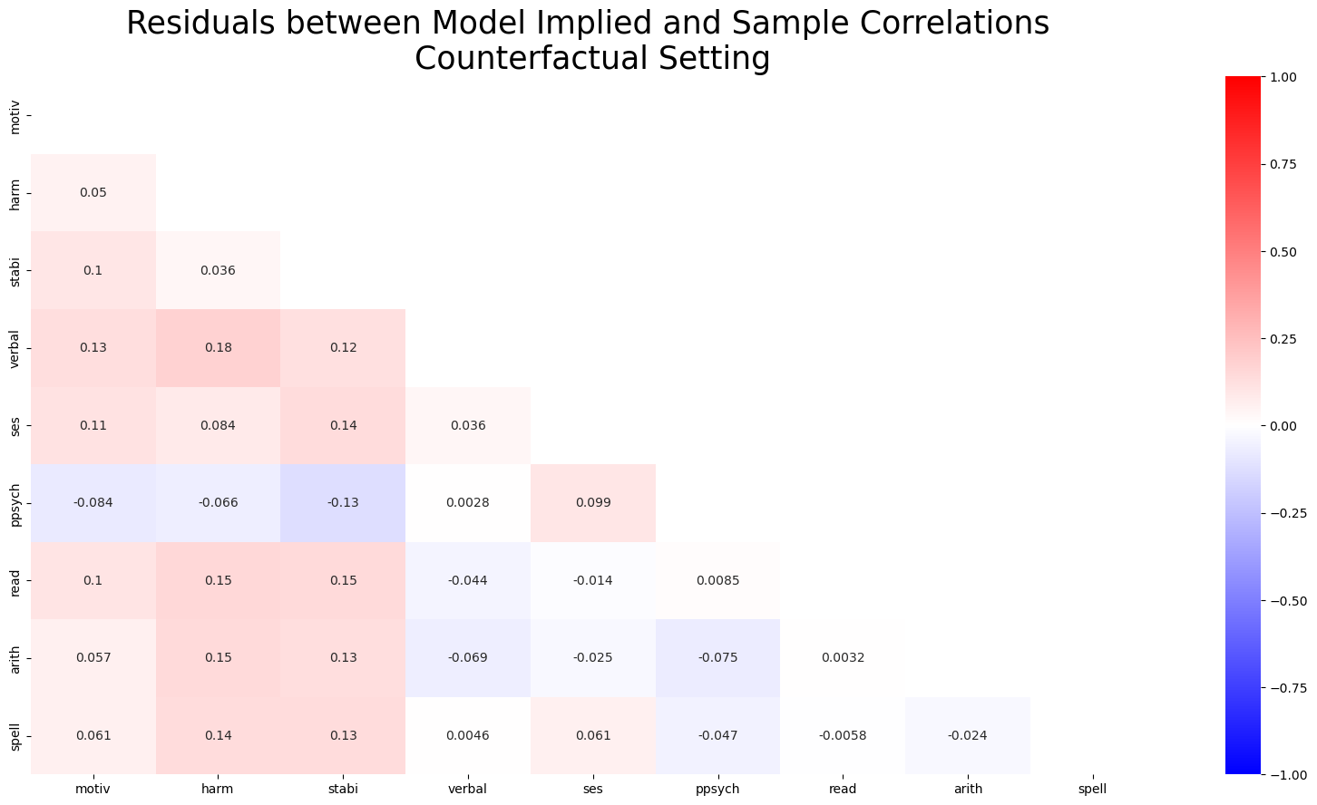
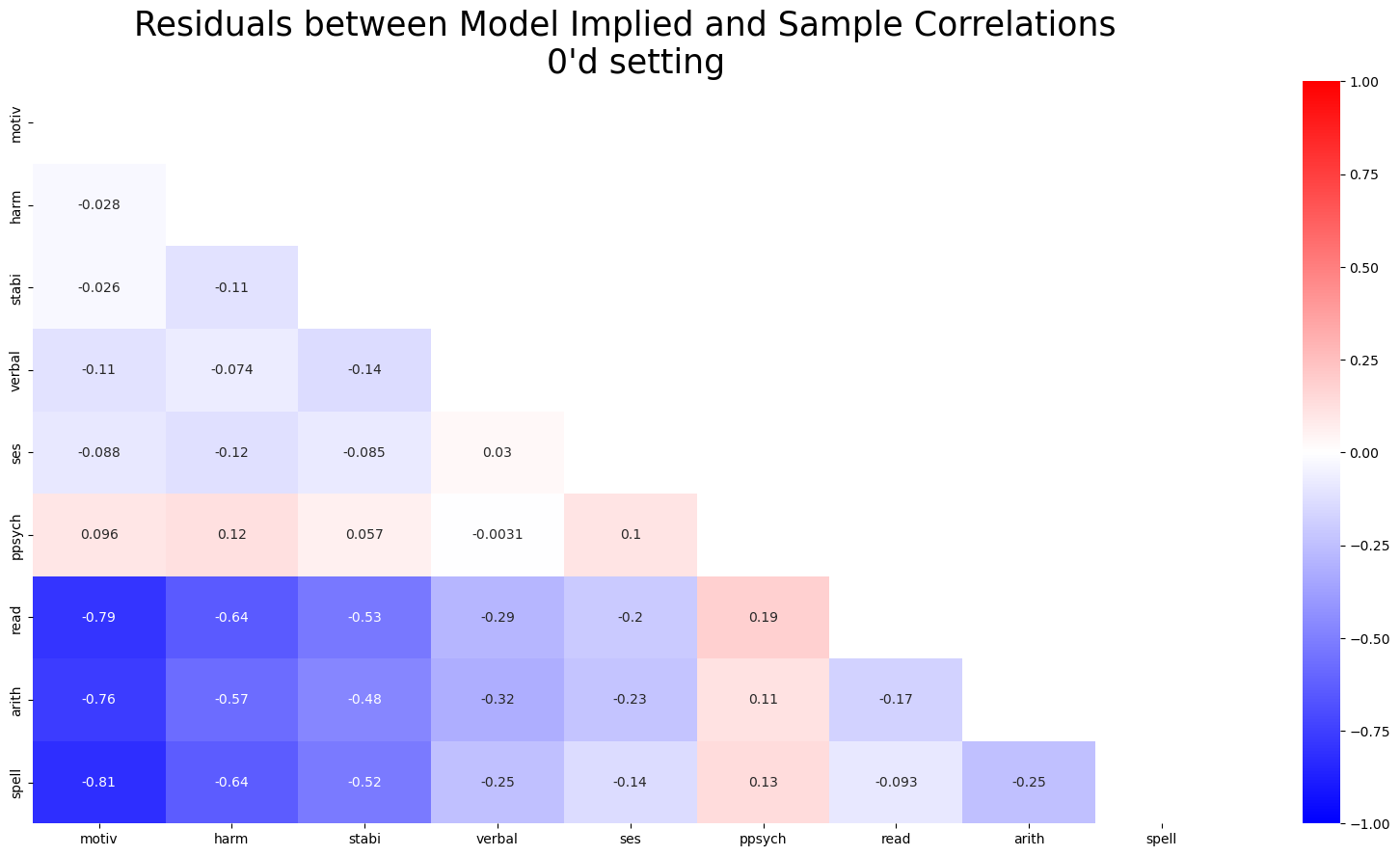
The plots are scaled identically here between -1 and 1. Highlighting significantly worse model fit under implausibly zero’d out beta coefficients.
Conclusion
Credibility versus Certification
“SEM is an inference engine that takes in two inputs, qualitative causal assumptions and empirical data, and derives two logical consequences of these inputs: quantitative causal conclusions and statistical measures of fit for the testable implications of the assumptions. Failure to fit the data casts doubt on the strong causal assumptions of zero coefficients or zero covariances and guides the researcher to diagnose, or repair the structural misspecifications. Fitting the data does not “prove” the causal assumptions, but it makes them tentatively more plausible.”
- Bollen and Pearl in Eight myths about causality and structural equation models