Examined Algorithms – theoreticalrisks

import pandas as pd
from matplotlib import pyplot as plt
import nltk
from sklearn.datasets import make_blobs
from sklearn.cluster import KMeans
from sklearn.metrics import silhouette_samples, silhouette_score
from factor_analyzer import FactorAnalyzer
from sklearn.decomposition import FactorAnalysis
import random
import seaborn as sns
random.seed(30)

Create the Fake Customer Purchase data

We create two fake data sets with a discernible structures, but we don’t want the models to work too easily so we sample again from these data pairing both sets as if we have a customer and their products.

X, y = make_blobs(n_samples=10000, 
                  centers=5, 
                  n_features=6,
                 random_state=0
                 )

prods = ['product_desc_' + str(x) for x in range(0, 6)]
df_products = pd.DataFrame(data=X, columns=prods)
df_products['Product_Class'] = y
df_products['Product_ID'] = df_products.index

X, y = make_blobs(n_samples=1000, 
                  centers=10,
                  n_features=8,
                  random_state=0)
custs = ['customer_desc_' + str(x) for x in range(0, 8)]
df_customer = pd.DataFrame(data=X,
                           columns=custs)

df_customer['Customer_Class'] = y
df_customer['Customer_ID'] = df_customer.index

# Randomly Select some of the customers to pair with random purchases
day1 = pd.DataFrame(zip(
        [random.randint(0, 1000) for x in range(0, 500)],
        [random.randint(0, 10000) for x in range(0, 500)]
        ), 
        columns=['Customer_ID', 'Product_ID']
                   )

day2 = pd.DataFrame(zip(
        [random.randint(0, 1000) for x in range(0, 500)],
        [random.randint(0, 10000) for x in range(0, 500)]
        ), 
        columns=['Customer_ID', 'Product_ID'])

purchases = pd.concat([day1, day2],
                      axis=0, 
                      ignore_index=True)
purchases.head()

	Customer_ID	Product_ID
0	552	773
1	827	8608
2	296	518
3	625	5394
4	30	8543

df_purchases = None
for purchase in range(0, len(purchases)):
    cust_id = purchases['Customer_ID'][purchase]
    prod_id = purchases['Product_ID'][purchase]
    cust = df_customer[df_customer['Customer_ID'] == 
                       cust_id]
    cust.reset_index(inplace=True, drop=True)
    prod = df_products[df_products['Product_ID'] == 
                       prod_id]
    prod.reset_index(inplace=True, drop=True)
    temp = pd.concat([prod, cust], axis=1)
    if df_purchases is None:
        df_purchases = pd.concat([prod, cust], axis=1)
    else:
        df_purchases = df_purchases.append(
            pd.concat([prod, cust], axis=1)
        )
df_purchases.reset_index(inplace=True, drop=True)
df_purchases

	product_desc_0	product_desc_1	product_desc_2	product_desc_3	product_desc_4	product_desc_5	Product_Class	Product_ID	customer_desc_0	customer_desc_1	customer_desc_2	customer_desc_3	customer_desc_4	customer_desc_5	customer_desc_6	customer_desc_7	Customer_Class	Customer_ID
0	-1.233276	8.747108	9.165746	-0.007541	4.652380	1.913970	1	773	-6.374916	-2.257586	7.688019	-7.992522	7.593467	-9.193683	10.376847	-0.388405	8.0	552.0
1	-0.170403	8.219852	9.710727	-1.550177	5.811414	1.492459	1	8608	9.294317	-2.231715	6.061894	-0.438840	1.246116	8.820684	-9.950039	-7.391761	1.0	827.0
2	-2.822567	8.036298	10.929105	-0.935760	6.077699	1.265250	1	518	-8.793580	4.805865	6.167272	5.770659	7.451190	4.144325	1.196351	5.414350	2.0	296.0
3	1.019780	6.766354	-9.152836	-8.611808	-8.749707	6.637419	2	5394	-7.047638	-2.131113	5.768863	-8.094387	6.223832	-8.834962	9.629384	-1.935227	8.0	625.0
4	4.321656	7.430975	8.847703	5.921750	-0.868445	5.483210	3	8543	-0.169121	1.346768	-10.211423	1.709859	1.655568	1.891809	7.856076	4.333816	4.0	30.0
...	...	...	...	...	...	...	...	...	...	...	...	...	...	...	...	...	...	...
995	2.151425	3.179085	2.337353	0.559543	-1.629433	2.493002	0	8383	-4.926378	-1.474424	2.848533	-10.733950	4.237231	5.048239	-5.263423	-7.005510	5.0	272.0
996	0.475735	4.378010	2.597665	1.569648	-1.131376	3.110801	0	6141	7.821350	-1.948967	6.039587	1.739432	2.351800	8.325224	-10.263796	-7.450850	1.0	616.0
997	4.621406	7.791088	8.592775	6.423716	0.915721	4.727899	3	406	-9.236352	2.760513	-7.290240	9.169618	-0.188279	-2.443252	-4.153840	6.140598	3.0	266.0
998	-1.720297	8.174031	9.746428	-1.849028	5.046019	0.951072	1	9737	-1.411479	0.830250	5.167232	-9.188249	3.176105	4.570698	-6.300042	-7.561958	5.0	263.0
999	2.804878	4.882689	-0.262516	0.311810	-1.867281	4.639076	0	3486	-6.696620	1.945182	-7.520248	8.545794	3.743541	-3.216961	-4.505348	3.400242	3.0	589.0

1000 rows × 18 columns

Preliminary Plotting: Do the Factors seperate the structure?

A worthwhile plot to apply with any dimensional reduction technique (such as PCA or factor analysis) is to check if and how the data seperates when plotted on the reduced plane. In lieu of knowledge of the data we can always compare this representation to the output of a clustering algorithm.

cust_desc = [x for x in df_purchases.columns if 
             'customer_desc' in x]
X = df_customer[cust_desc]
kmeans = KMeans(init='k-means++',
                n_clusters=3, 
                n_init=30
               )
kmeans.fit(X)
clusters = kmeans.predict(X)
X['cluster'] = clusters

sklearn_fa = FactorAnalysis(n_components=2, 
                            rotation='varimax'
                           )
Y_fa = pd.DataFrame(sklearn_fa.fit_transform(X[cust_desc]))
X = pd.concat([X, Y_fa], axis=1)
X[[0, 1, 'cluster']].plot.scatter(x=0,
                      y=1,
                      c='cluster',
                      colormap='viridis')
plt.title("Factor Analysis Representation - Coloured by inferred Clusters")
plt.ylabel("Factor 1")
plt.xlabel("Factor 2")
plt.style.use('default')
plt.show()

/Users/nathanielforde/.local/lib/python3.6/site-packages/ipykernel_launcher.py:9: SettingWithCopyWarning: 
A value is trying to be set on a copy of a slice from a DataFrame.
Try using .loc[row_indexer,col_indexer] = value instead

See the caveats in the documentation: https://pandas.pydata.org/pandas-docs/stable/user_guide/indexing.html#returning-a-view-versus-a-copy
  if __name__ == '__main__':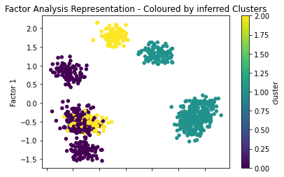

We can see here that the factors do a pretty good job of seperating the classes (0, 1), but mix up (2, 1). In addition we can see that there are 7 distinct clusters on the factor analysis representation which suggests that our choice three clustering classes is too low.

Choosing the number of Factors

One suggestive way in which to determine the number of factors which we should extract is to build the skree plot of the eigenvalues and select the number of features where there is a higher relative eigenvalues.

import numpy as np
feature_names = ['customer_desc_' + str(x) for x in range(0, 8)]

fa = FactorAnalyzer(n_factors=3)
fa.fit(X[feature_names], 10)
ev, v = fa.get_eigenvalues()
plt.plot(range(1,X[feature_names].shape[1]+1),ev)
plt.show()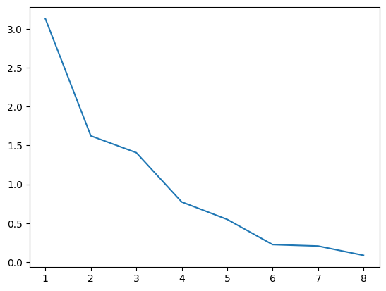

On the basis of this plot we should probably choose no more than two factors at most but we’ll continue with 3 for purposes of illustration. The factor loadings are linear functions of the observed features and so we may interpret the newly created factors by observing which of the observed features play a greater role in their composition.

fa_loading_matrix = pd.DataFrame(fa.loadings_, 
                                 columns=['FA{}'.format(i) for 
                                          i in range(1, 3+1)], 
                              index=feature_names)
fa_loading_matrix['Highest_loading'] = fa_loading_matrix.idxmax(axis=1)
fa_loading_matrix = fa_loading_matrix.sort_values('Highest_loading')
fa_loading_matrix

	FA1	FA2	FA3	Highest_loading
customer_desc_1	0.727724	0.024771	0.091443	FA1
customer_desc_3	0.826998	0.068252	0.014691	FA1
customer_desc_5	0.637687	-0.003234	0.489801	FA1
customer_desc_7	0.787048	0.081877	-0.414776	FA1
customer_desc_4	0.015911	1.001115	0.175406	FA2
customer_desc_6	-0.172587	0.077989	-0.684129	FA2
customer_desc_0	-0.229668	-0.628541	0.355323	FA3
customer_desc_2	-0.304156	0.217303	0.440891	FA3

We can see here that there is probably only one sensible factor to be derived from our dataset.

import seaborn as sns

plt.figure(figsize=(25,5))

# plot the heatmap for correlation matrix
ax = sns.heatmap(fa_loading_matrix.drop('Highest_loading', axis=1).T, 
                vmin=-1, vmax=1, center=0,
                cmap=sns.diverging_palette(220, 20, n=200),
                square=True, annot=True, fmt='.2f')

ax.set_yticklabels(
    ax.get_yticklabels(),
    rotation=0);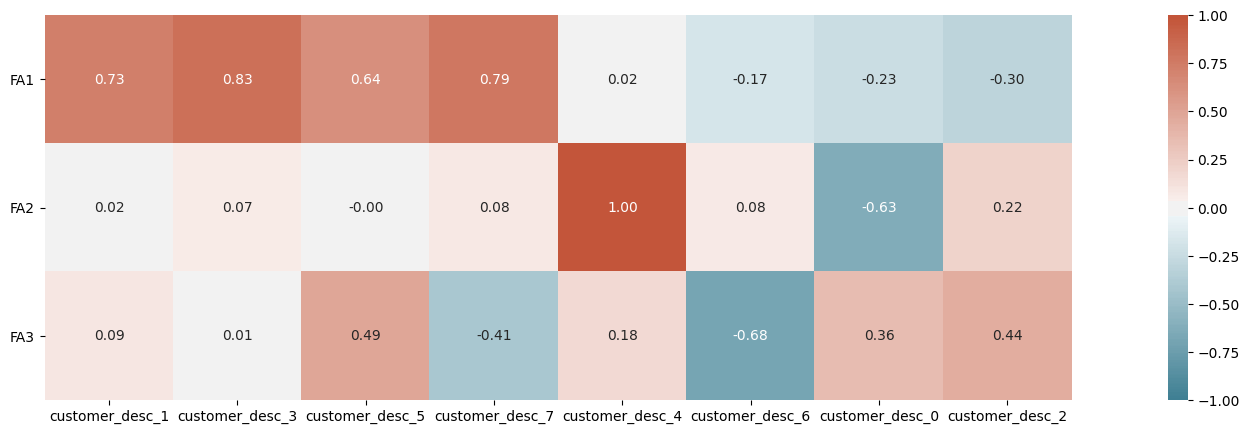

communalities = pd.DataFrame(fa.get_communalities(), 
                             index=list(feature_names))
features_comm = list(communalities[communalities[0] > 0.33].index)
print('Total variables/features with communalities >0.33: {}'.format(len(features_comm)))
communalities

Total variables/features with communalities >0.33: 8

	0
customer_desc_0	0.574065
customer_desc_1	0.538558
customer_desc_2	0.334116
customer_desc_3	0.688800
customer_desc_4	1.033252
customer_desc_5	0.646560
customer_desc_6	0.503901
customer_desc_7	0.798188

Testing the Validity of a Hypothetical Factor

Cronbach’s Alpha is a statistical measure of the reliability of the factor analysis derived from a test of the covariances matrix of features which make up the proposed latent factor. A cronbach alpha closer to 1 is desired.

\(\alpha = \frac{K}{K-1}\left(1-\frac{\sum \sigma^2_{x_i}}{\sigma^2_T}\right)\)

where

\(\sigma^2_T = \sum \sigma^2_{x_i} + 2 \sum_{i < j}^K {\rm cov}(x_i,x_j)\)

a combination of the observational measure of variance and inter-metric covariances for each observational variable. This ties this measure to the Factor analysis model since the covariances can be re-expressed in terms of the factor loadings.

\(\sigma^2_T = \sum \sigma^2_{x_i} + 2 \sum_{i < j}^K (l_{i, 1} + \epsilon_{i})(l_{j, 1} + \epsilon_{j})\)

which means that if the factors loadings are fairly high relative the the random components of the variance then we’ll get a ratio that come close to one. Conversely low loadings will ensure that the denominator drags the ratio down.

import numpy as np

def CronbachAlpha(observed_measures):
    observed_measures = np.asarray(observed_measures)
    sample_vars = observed_measures.var(axis=1, ddof=1)
    total_scores = observed_measures.sum(axis=0)
    nitems = len(observed_measures)

    return nitems / (nitems-1.) * (1 - sample_vars.sum() / total_scores.var(ddof=1))

#Collate the observed features

factor1 = [X['customer_desc_1'], X['customer_desc_3'], 
             X['customer_desc_5'], X['customer_desc_7']]

factor2 = [X['customer_desc_4'], X['customer_desc_0']]

factor3 = [X['customer_desc_5'], X['customer_desc_6'], 
             X['customer_desc_2']]
#Get cronbach alpha
factor1_alpha = CronbachAlpha(factor1)
#factor2_alpha = CronbachAlpha(factor2)
#factor3_alpha = CronbachAlpha(factor3)
print(factor1_alpha, 
      factor2_alpha, 
      factor3_alpha
     )

0.7889764629492505 -3.382959230225132 -0.8158399732248119

Which shows as expected that only one of the proposed factors is sensible.