Survival Regression Models in PyMC
Time to Attrition in People Analytics
2023-12-30
Layered Abstractions and Hyperobjects

Concepts that defy easy panoptic survey prohibit easy action e.g. climate change and mathematical structures such as families of probability distributions
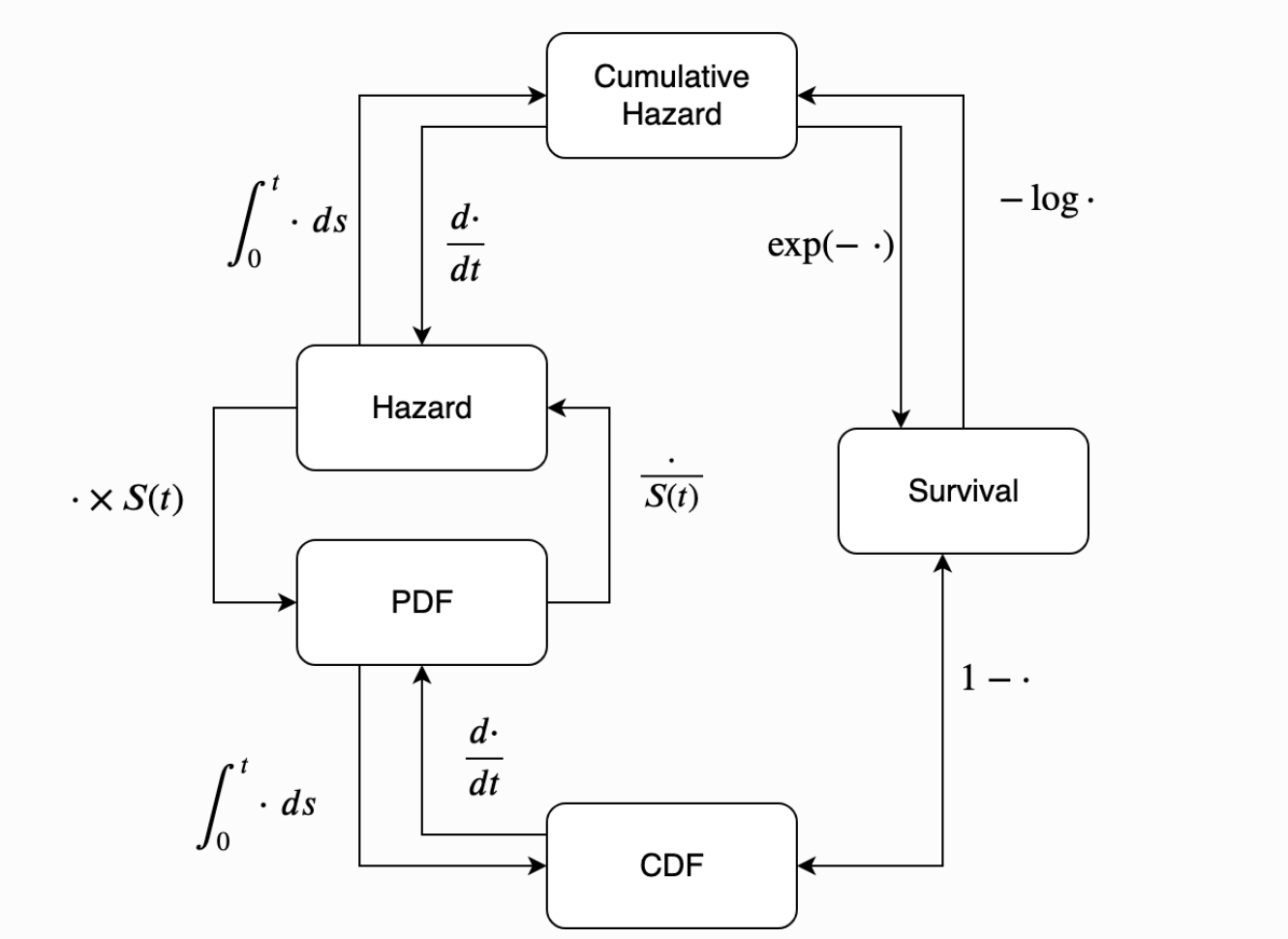
Perspectives on Probability
Top-Down and Abstract
\[ h(t) = \frac{f(t)}{S(t)} \\ H(t) = -ln(S(t))\]
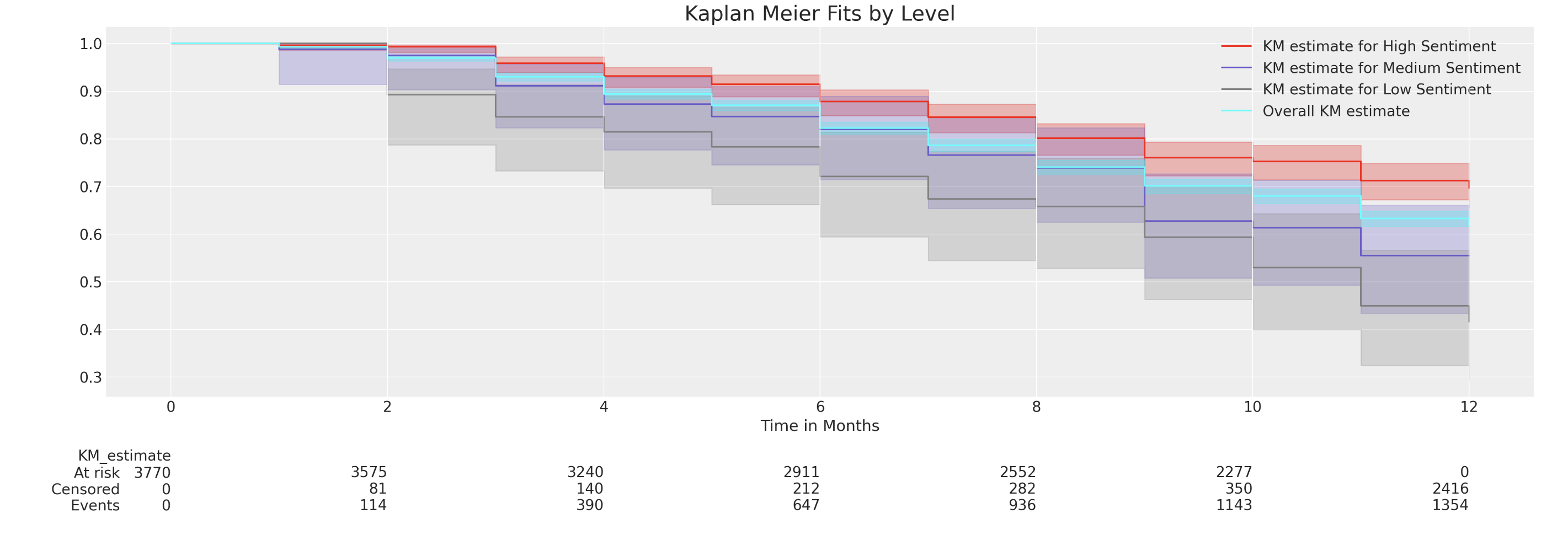
Actuarial Tables and Survival Curves
Bottom-Up and Concrete
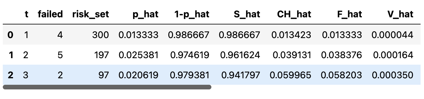
Actuarial Tables try to estimate CDF and Survival functions
Calculation of these abstract quantities proceeds from a clear and concrete notion of the risk-set in time.
Time to Attrition Data
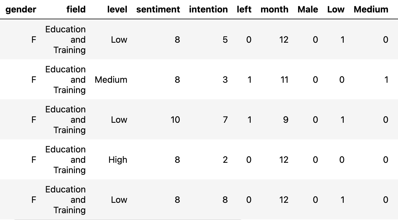 Question: What is the relationship between individual characteristics and their expected survival times?
Question: How do individual survival times vary as a function of the levels in their covariates.
Regression for Survival Times
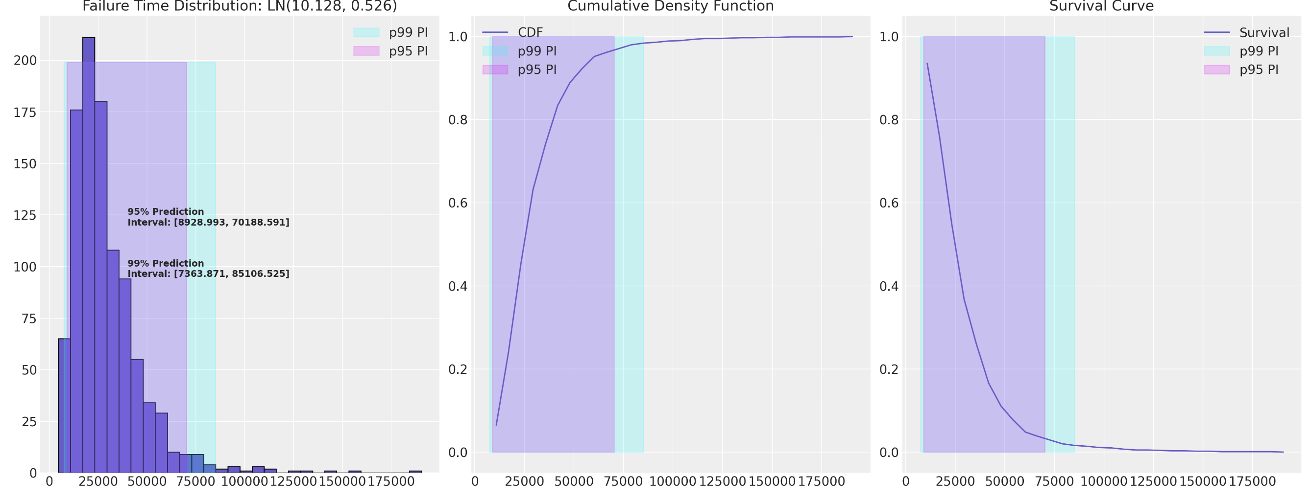
Distributions for Modelling Attrition
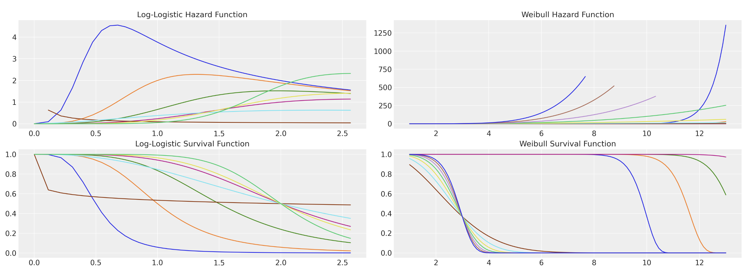
Monotonoc or non-monotonic hazards determined by distribution choice. Risk spikes important in early periods of employment.
Parametric Model Structure
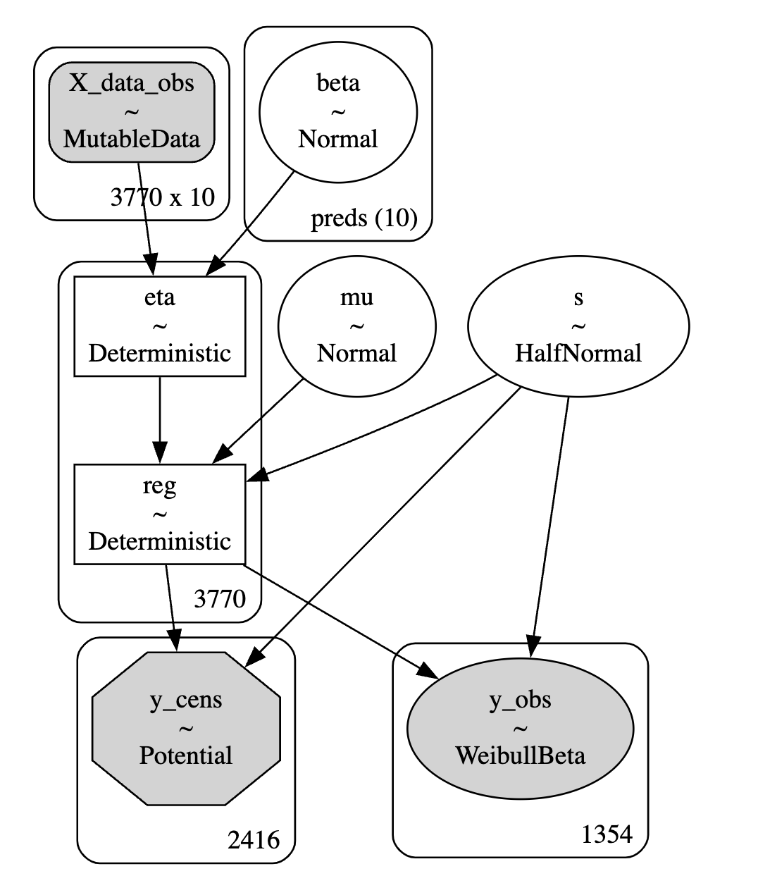
Accelerated Failure time models incorporate the regression component as a weighted sum that enters the parametric probability model
For instance: \[ Weibull(\alpha, \beta) \\ = Weibull(\alpha, reg)\]
Proportional Hazards Cox Regression
“There’s the ‘mañana paradox’: the unwelcome task which needs to be done, but it’s always a matter of indifference whether it’s done today or tomorrow; the dieter’s paradox: I don’t care at all about the difference to my weight one chocolate will make.” - Dorothy Edgington
Proportional Hazards Cox Regression
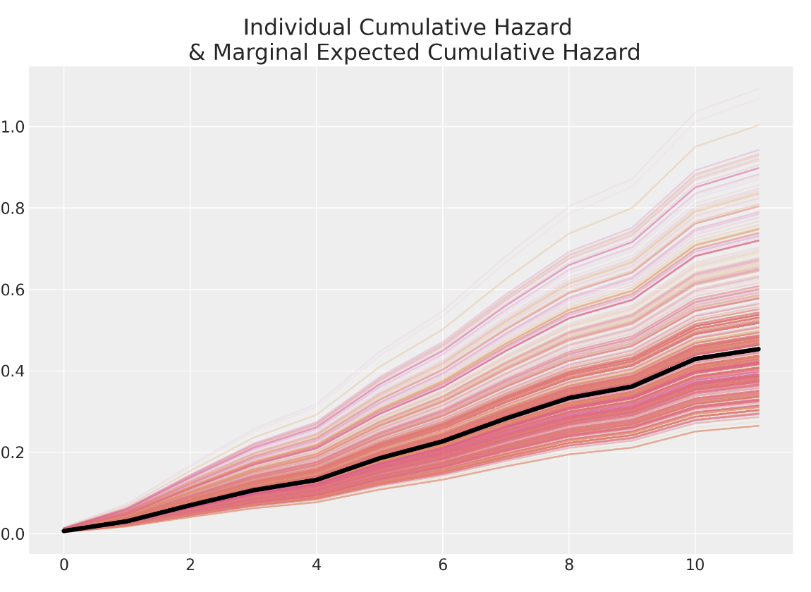
Cumulative Hazard across Individuals
Proportional Hazards Cox Regression
Using the Poisson Trick
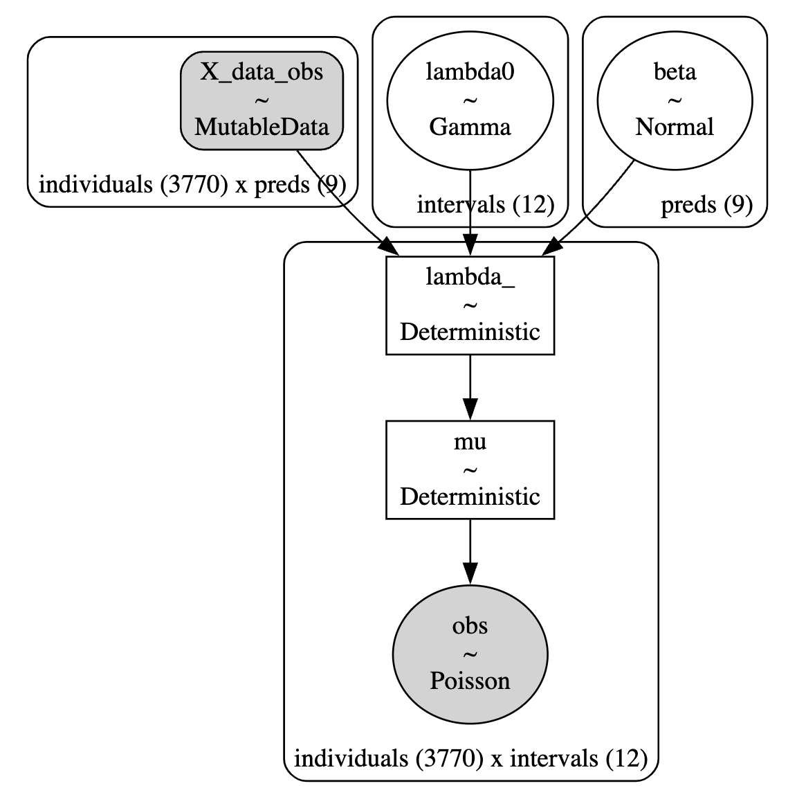
\[ CoxPH(left, month) \sim gender + level \]
is akin to
\[ left \sim glm(gender + level + (1 | month)) \\ \text{ where link is } Poisson \]
applying an offset to the event rate for each time interval.
Comparing Models
Stated Intention and Sentiment
\[ CoxPH(left, month) \sim gender + field + level + sentiment \]
\[ CoxPH(left, month) \sim gender + field + level + sentiment + intention \]
Comparing Models
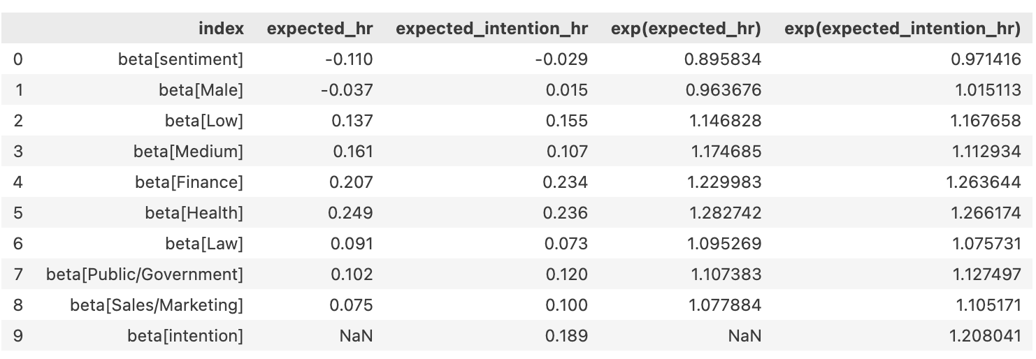
Interpreting Model Coefficients
- If \(exp(\beta)\) > 1: An increase in X is associated with an increased hazard (risk) of the event occurring.
- If \(exp(\beta)\) < 1: An increase in X is associated with a decreased hazard (lower risk) of the event occurring.
- If \(exp(\beta)\) = 1: X has no effect on the hazard rate.
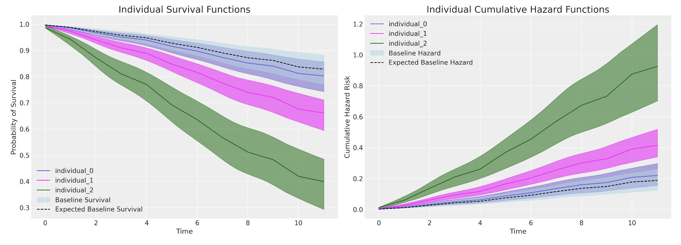
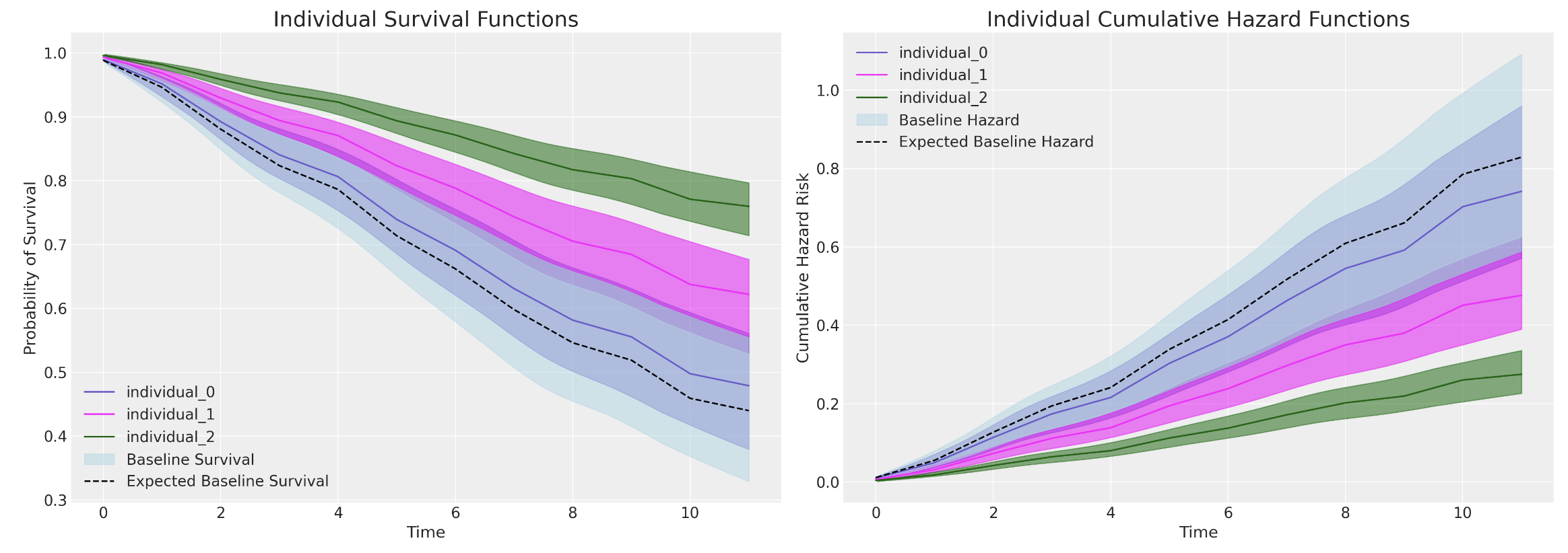
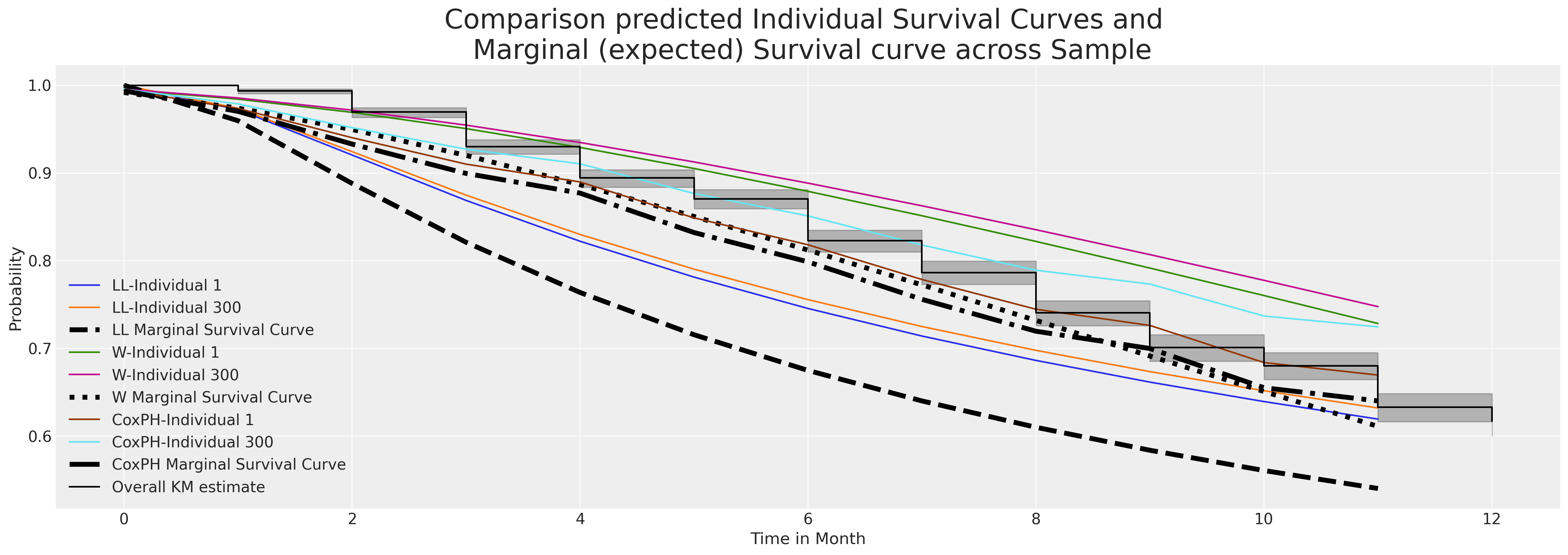
Predicting Marginal Effects 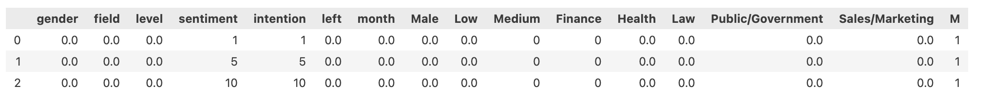
Comparing Models
Predicting Marginal Effects
Comparing Models
AFT models allow us to quantify the acceleration factor due to an individual or group’s risk profile.
Comparing Models
Marginal Survival Functions and WAIC

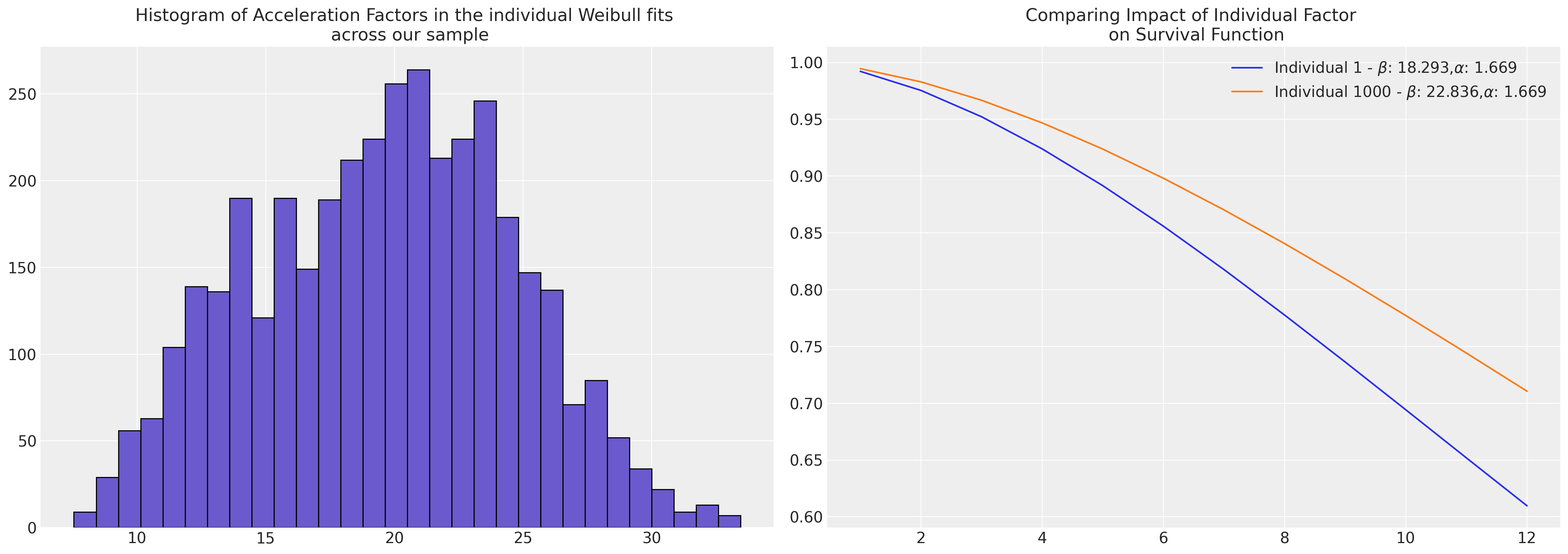
Frailty Models and Individual Heterogeneity
We want to relax the assumptions of Cox Proportional Hazards model. We introduce (i) frailty terms and (ii) stratified risks
\[ \lambda_{i}(t) = \color{green}{z_{i}}exp(\beta X)\color{red}{\lambda_{0}^{g}(t)} \]
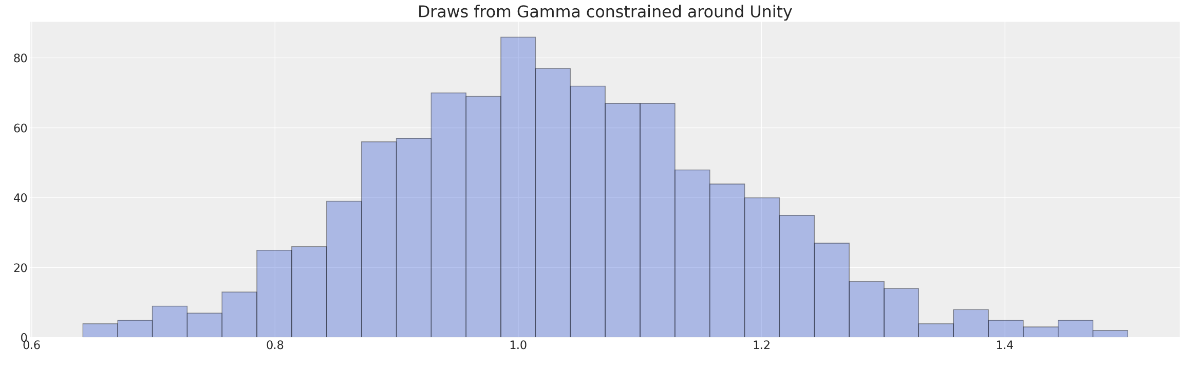
The multiplicative frailty terms \(z_{i}\) can be specified as a gamma distribution centred on unity with stratified risks
Frailty Model Structure
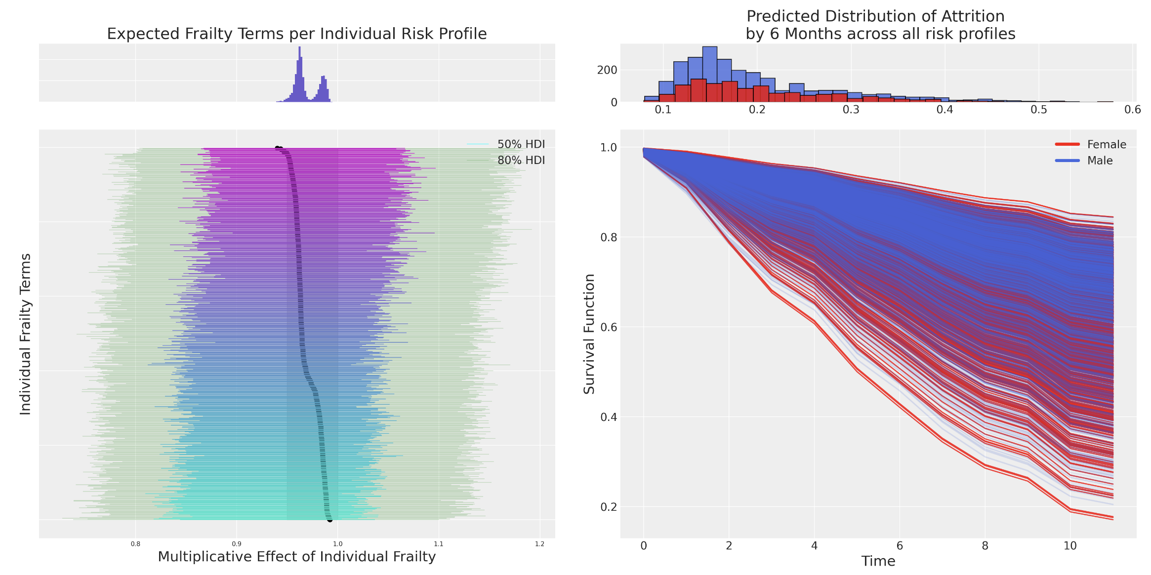
Individual Frailties

Frailty Model Structure
Shared Frailties

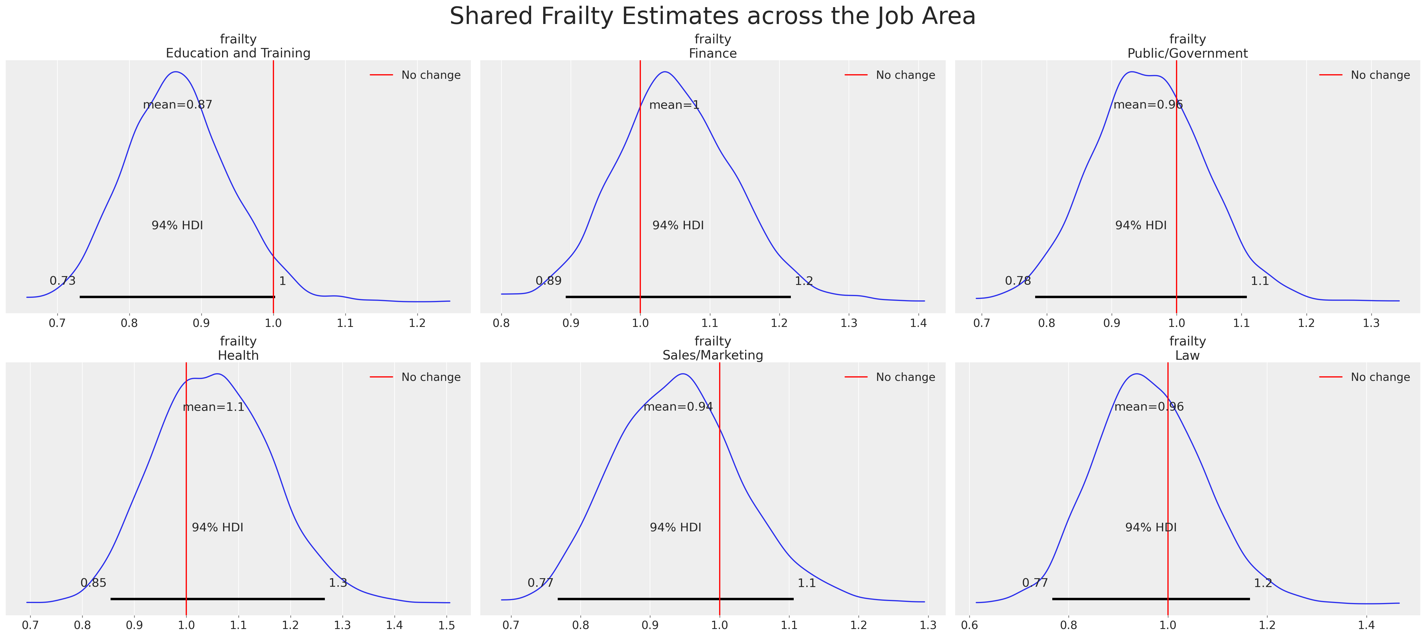
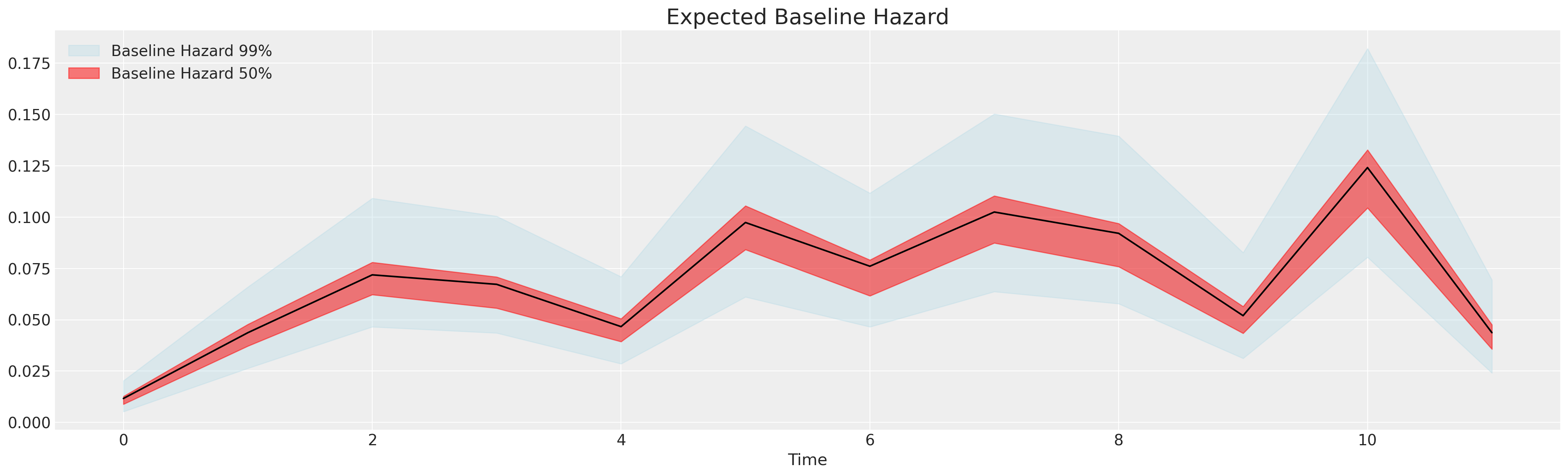
Frailty Models and Stratified Baseline Risks

We see differences in the risks stratified by gender and additionally how the magnitude of the baseline hazard shrinks with more or less well-specified covariate in the model.
Individual Frailties and Marginal Statistics
Conclusion
- Survival Analysis is a tool for the expression of probabilities governing state-transitions
- Important everywhere process efficiency and transformative outcomes matter. Corrects for censorship bias of naive summaries.
- Allows for sophisticated expression of risk over time and along many dimensions. Variety of hierarchical modelling options
- Bayesian estimation of these complex model structures is natural and informative. Meaningful across a range of disciplines and domains.
- Provides an actionable lens on “actuarial” risk and “diagnostic” causal analysis in time.