Bayesian Structural Causal Inference

Exploring Space, Finding Structure, Testing Robustness

Nathaniel Forde

Data Science @ Personio Open Source Contributor @ PyMC

Preliminaries

Who am I?

• I’m a data scientist at Personio
  • Bayesian statistician,
  • Reformed philosopher and logician.
• Website: https://nathanielf.github.io/

Code or it didn’t Happen

The worked examples used here can be found here

My Website

Who Should Care About This?

You’re in the right place if you’re asking:

• “Did our intervention actually work, or did selection bias fool us?”
• “How sensitive are our conclusions to unobserved confounding?”
• “Can we simulate policy changes before deploying them?”
• “Which variables truly matter for our causal story?”

You’ll need familiarity with:

• Basic causal inference (treatment effects, confounding)
• Regression modeling (OLS, interpreting coefficients)
• Bayesian thinking (priors, posteriors, uncertainty)
• Some Python/PyMC (though concepts transfer)

The Promise

By the end, you’ll understand how to systematically explore causal uncertainty rather than just hoping your assumptions hold.

The Pitch: World-Building Matters

Scientific success hinges on understanding that outcomes are driven by hidden structures, unobserved correlations, and selection mechanisms.

Structural causal modelling allows you to simulate system interventions safely, mapping the multiverse of potential outcomes to find the one world where your strategy actually works, and quantify where it might.

Agenda

• The Metaphor: The Physics of the Fish Tank
• The Invisible Threat: Hidden Confounding and \(\rho\)
• The Pruning: Variable Selection as World Elimination
• The Pitfalls: Why Total Flexibility Destroys Identification
• The Navigation: Mapping the Multiverse of Results

The Metaphor

The Pet Shop Problem

A causal analyst is like a pet-shop owner introducing a new fish to an aquarium.

The Question: “Does this fish survive?”

Wrong Focus: The fish’s intrinsic properties (the “Treatment” in isolation).

Right Focus: The physics of the tank—pH, predators, currents (the “Structural” environment).

The Insight

“What is the causal effect?” really asks:

“In which world are we operating?”

Two Philosophies of the Tank

Design-Based Minimalism

Philosophy: Find a “clean” corner of the tank (Natural Experiments).

Strength: Robust to local errors.
Limitation: If the whole tank is cloudy, you’re blind.

Structural Maximalism

Philosophy: Model the pumps, filters, and chemistry explicitly.

Strength: Explains why the fish survives.
Limitation: If the physics model is wrong, the prediction fails.

The Bayesian Commitment: We don’t know the exact physics. We use data to eliminate impossible tank setups and explore the plausible ones.

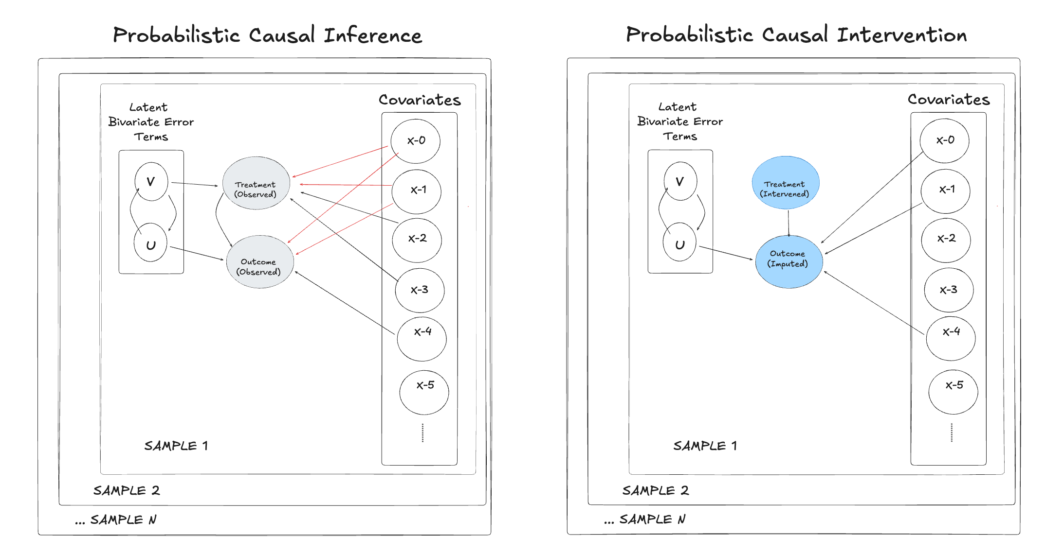
Joint Structural Modelling

The Mechanics of “The Tank”

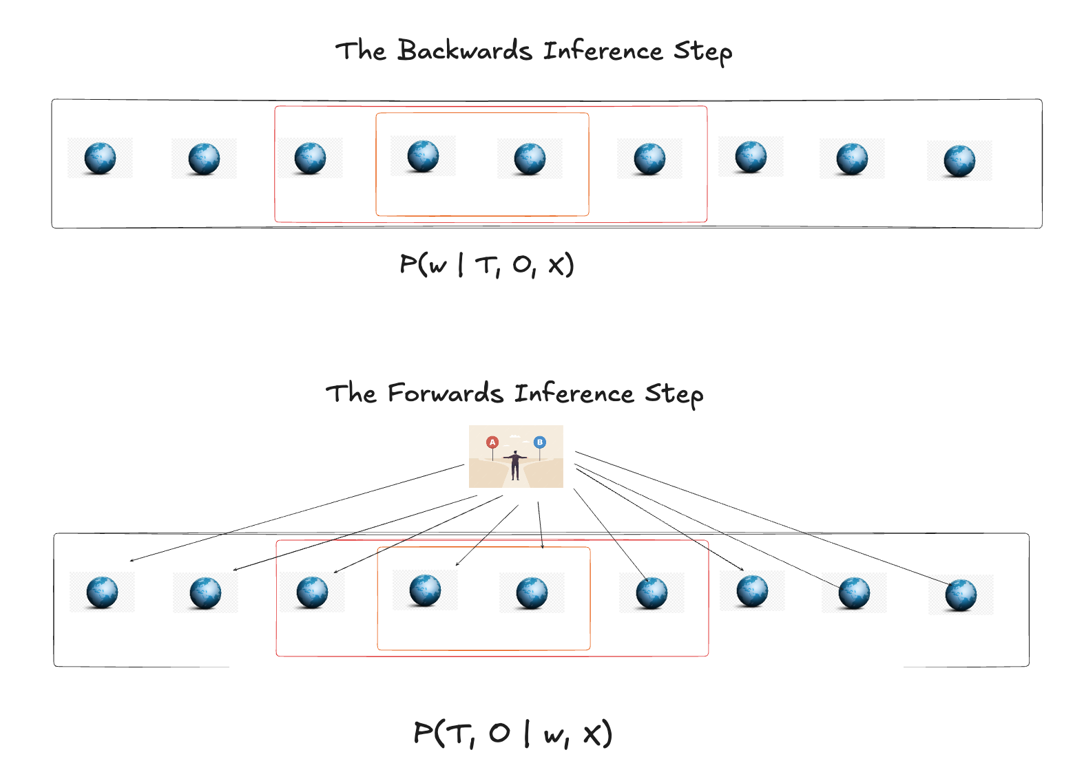
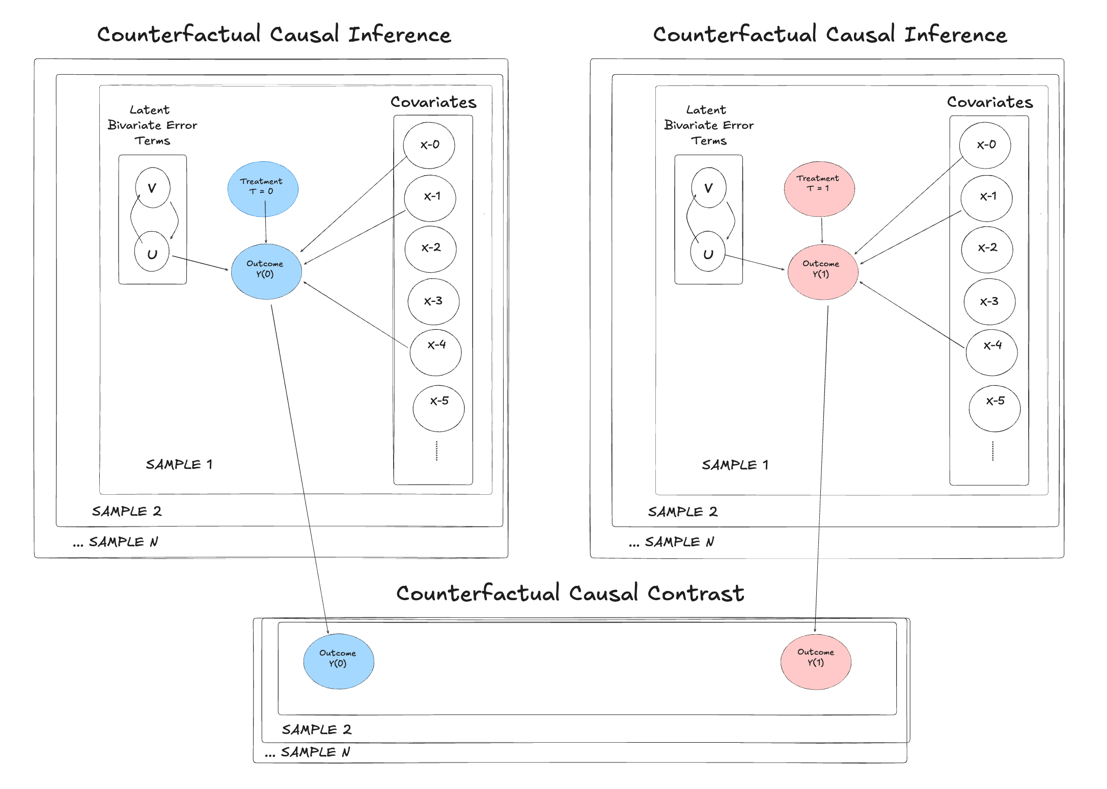
The Two Movements of Inference

Causal inference in a structural framework is a two-step dance:

1. Backwards (Inference): Use observed Treatment (\(T\)) and Outcome (\(Y\)) to infer the hidden state of the world (\(w\)).
2. Forwards (Counterfactual): Use that world state to simulate what would happen if we changed \(T\).

The Core Structural Model

Instead of treating treatment as exogenous, we model the joint data-generating process:

Outcome Equation:

\[Y_i = \alpha T_i + \beta' X_i + U_i\]

• \(\alpha\) = causal effect (what we want)
• \(X_i\) = observed covariates
• \(U_i\) = unobserved factors affecting outcome

Treatment Equation:

\[T_i = \gamma' Z_i + V_i\]

• \(Z_i\) = variables predicting treatment selection
• \(V_i\) = unobserved factors affecting treatment choice

The Key Question:

Are \(U_i\) and \(V_i\) correlated?

\[\text{Cov}(U_i, V_i) = \rho \sigma_U \sigma_V\]

• If \(\rho = 0\): Traditional methods work fine
• If \(\rho \neq 0\): We have hidden confounding

Important

This is what OLS assumes away. We’re going to estimate it instead.

The Invisible Threat: Hidden Correlation

The confounding isn’t just in what we measure—it’s in the covariance of the errors:

\[ \begin{pmatrix} U \\ V \end{pmatrix} \sim N\left(0, \begin{bmatrix} \sigma_U^2 & \rho\sigma_U\sigma_V \\ \rho\sigma_U\sigma_V & \sigma_V^2 \end{bmatrix}\right) \]

• \(\rho = 0\): The OLS assumption. \(T\) is “as-if” random.
• \(\rho \neq 0\): The Structural reality. Selection bias is modeled as a parameter.

The Bias is Real: OLS Drift

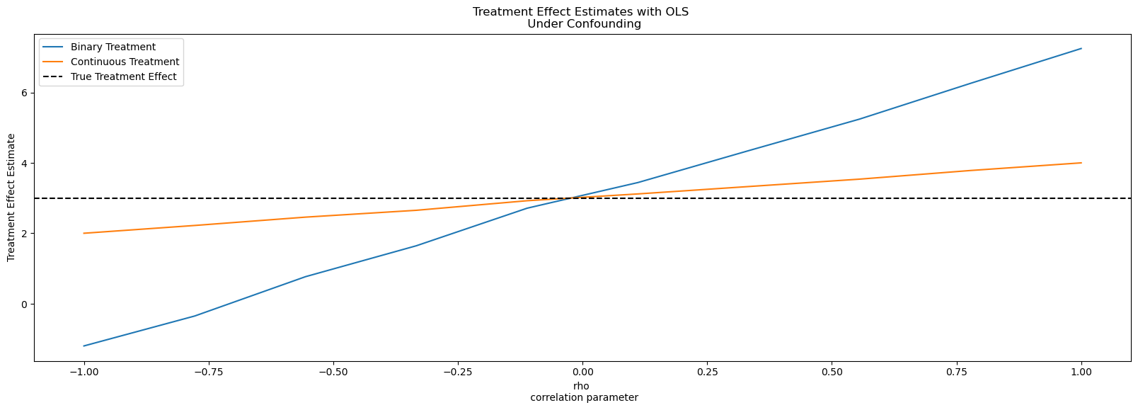
OLS estimates drift as ρ varies

If we ignore \(\rho\), our estimate of the effect (\(\alpha\)) is a ghost. It’s not just “noisy”—it’s fundamentally misplaced because we’ve ignored the unobserved “currents” in the tank.

Finding Structure (Pruning)

Discovering Structure as World Elimination

How do we find the “right” tank physics? We use Variable Selection Priors to collapse the multiverse.

Spike-and-Slab

The Sieve: It forces coefficients to be exactly zero or significantly non-zero.

Result: Eliminates worlds where irrelevant variables act as noise.

Horseshoe

The Funnel: It provides global and local shrinkage.

Result: Progressively prunes weak “paths” in the causal graph until only the strongest structural links remain.

Variable Selection Priors and Instrument Discovery

Navigating the Multiverse (Exploration)

Wrong turns in the Multiverse

The BART Pitfall

Using “Infinite Flexibility” (BART/GPs) in the Outcome equation is dangerous.

Why? If the model can explain \(Y\) through any arbitrary “wiggle,” it will “soak up” the causal signal.

• Outcome Flexibility: The model hides the effect of \(T\) inside the flexibility of the curve. \(\alpha\) becomes unidentifiable.
• Treatment Flexibility: Safe. It helps us model the “selection” process more accurately without obscuring the causal link.

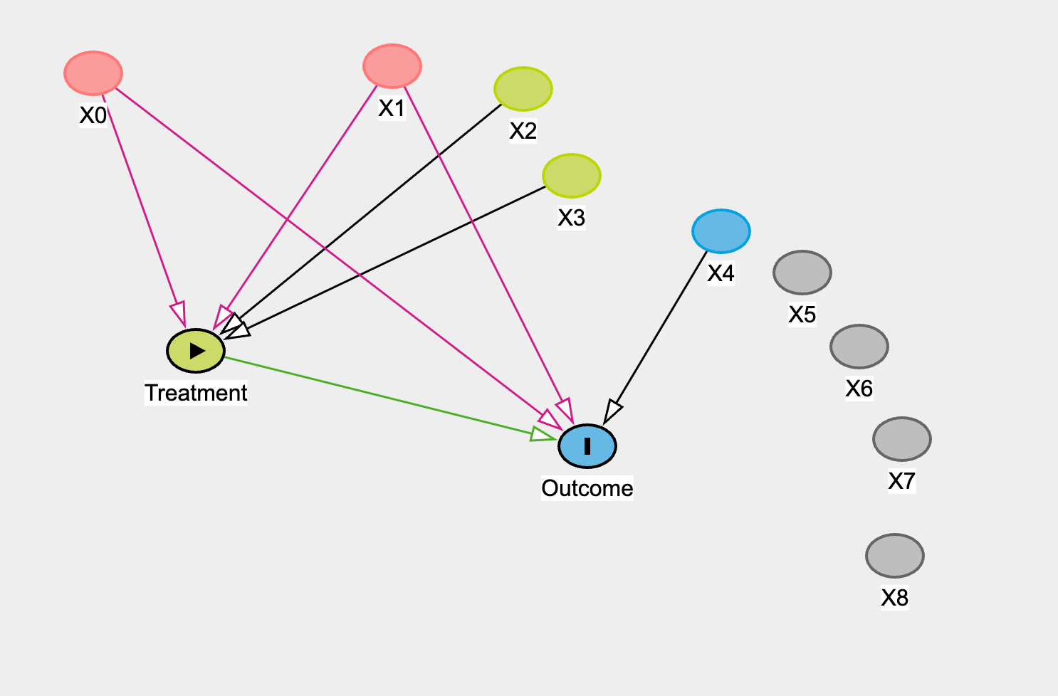
Identification Denied

BART outcome model absorbs the structural distinction between treatment and other covariates, rendering the treatment effect surplus to purpose. The signal is swallowed by the noise-handler.

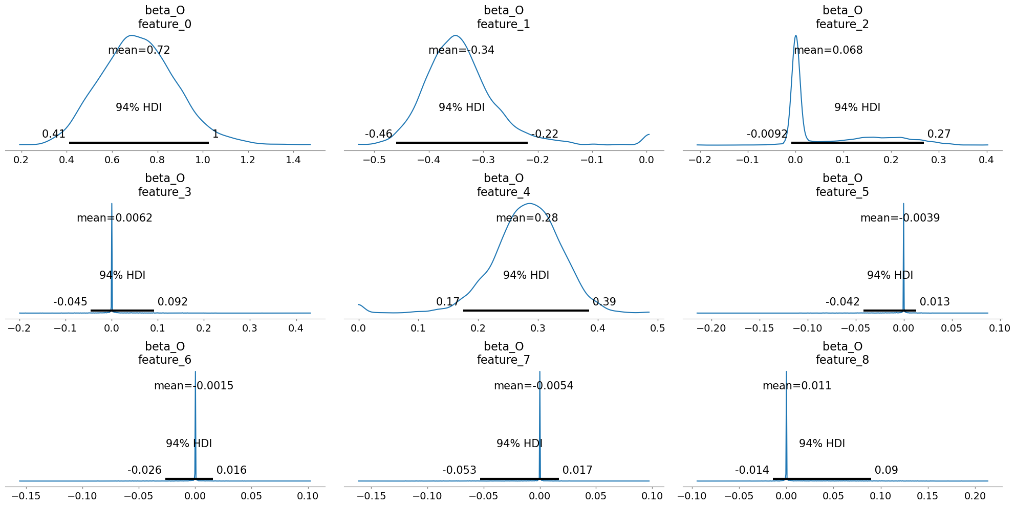
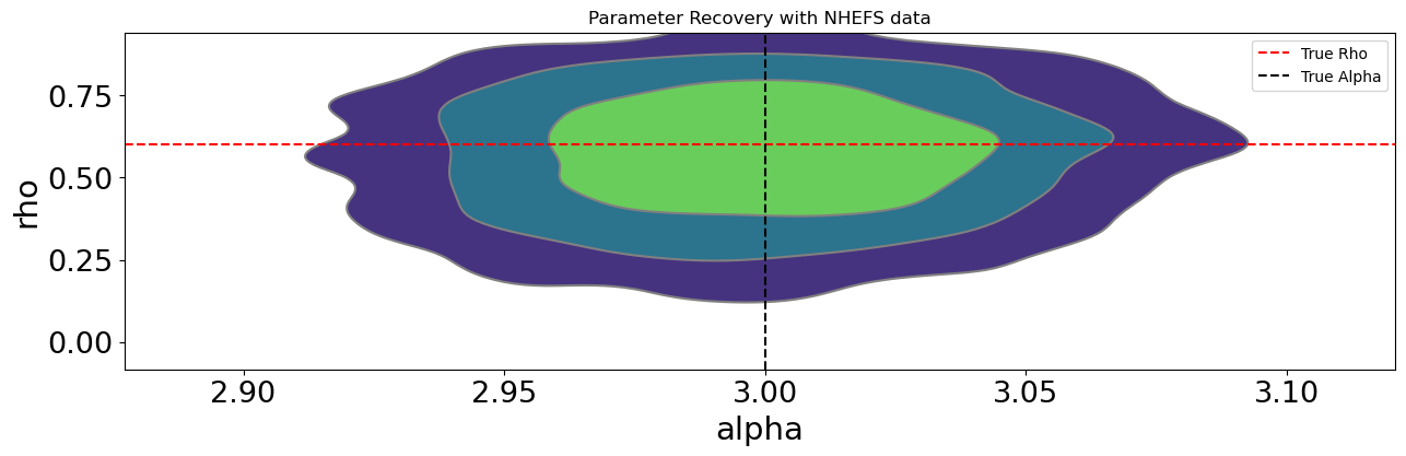
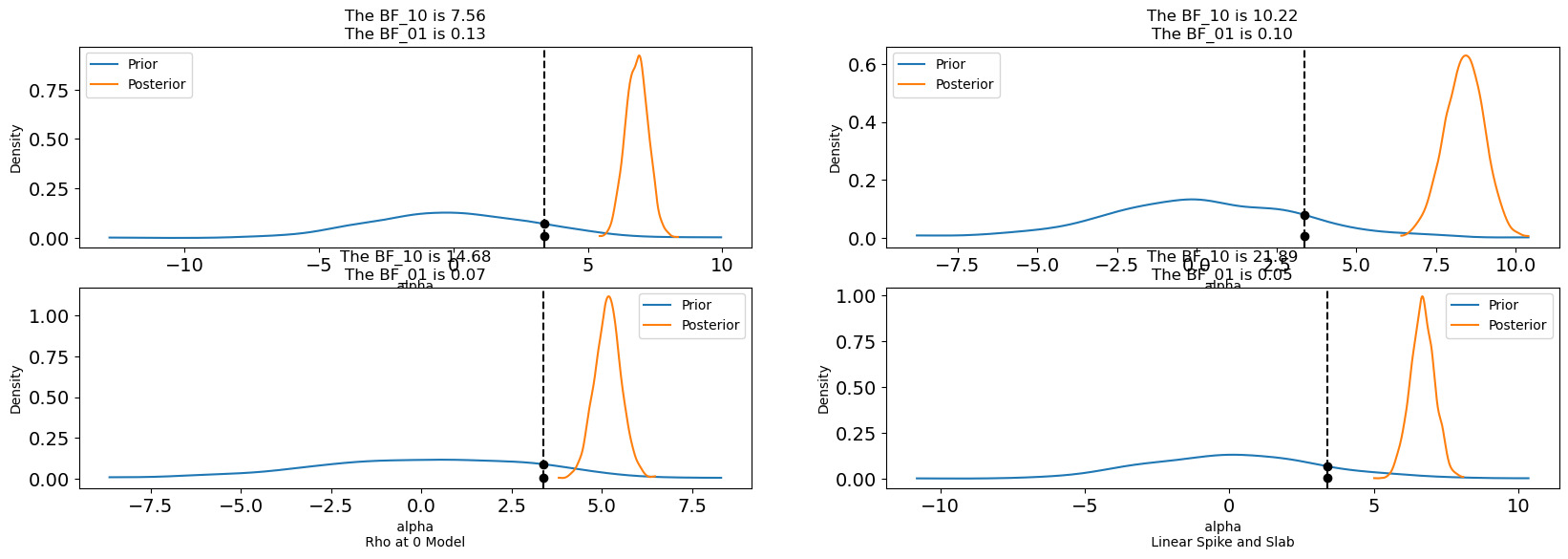
Parameter Recovery

fixed_parameters = {
    "rho": 0.6,
    "alpha": 3,
    "beta_O": [0, 1, 0.4, 0.3, 0.1, 0.8, 0, 0, 0, 0, 0, 0, 3, 0],
    "beta_T": [1, 1.3, 0.5, 0.3, 0.7, 1.6, 0, 0.4, 0, 0, 0, 0, 0, 0],
}
with pm.do(nhefs_binary_model, fixed_parameters) as synthetic_model:
    idata = pm.sample_prior_predictive(
        random_seed=1000
    )  # Sample from prior predictive distribution.
    synthetic_y = idata["prior"]["likelihood_outcome"].sel(draw=0, chain=0)
    synthetic_t = idata["prior"]["likelihood_treatment"].sel(draw=0, chain=0)
# Infer parameters conditioned on observed data
with pm.observe(
    nhefs_binary_model,
    {"likelihood_outcome": synthetic_y, "likelihood_treatment": synthetic_t},
) as inference_model:
    idata_sim = pm.sample_prior_predictive()
    idata_sim.extend(pm.sample(random_seed=100, chains=4, tune=2000, draws=500))

Identification Achieved

Core Principle

Flexibility (capturing complex patterns) and Identification (isolating causal effects) are in tension. Structure the role flexible models well in causal inference.

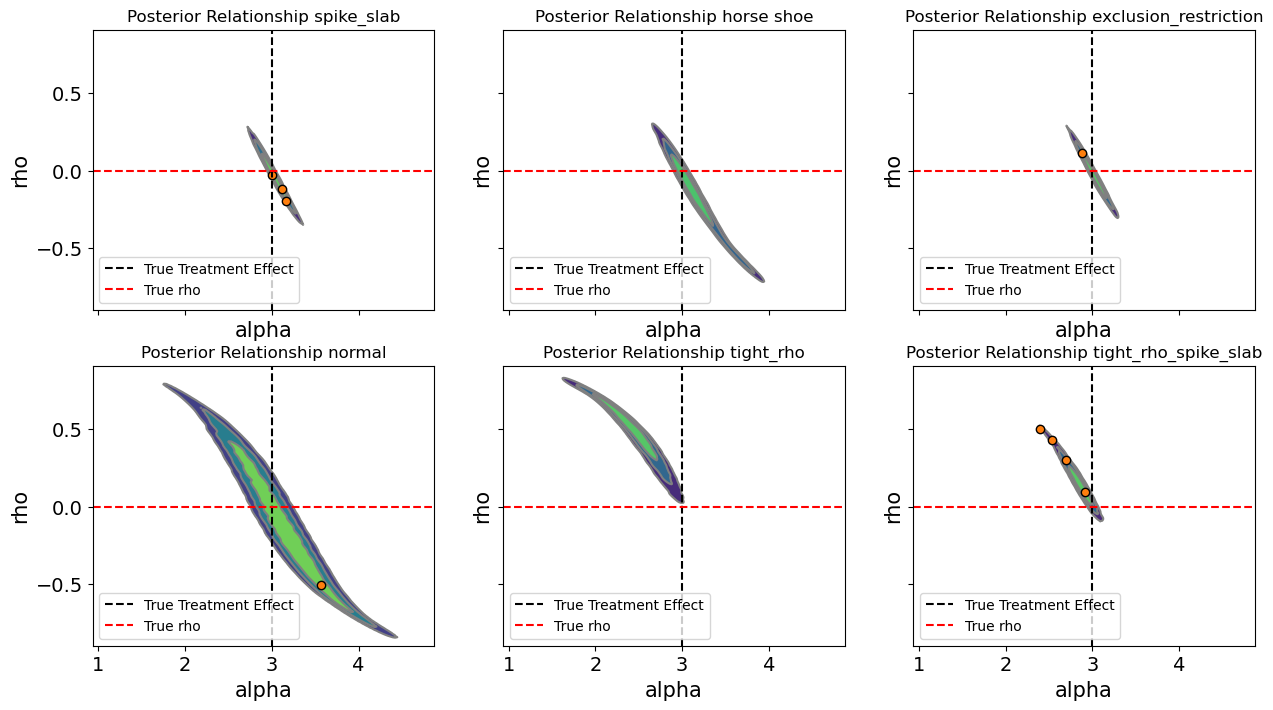
Mapping the Multiverse

We don’t estimate a point; we map a territory.

# We explore different 'Universes' of confounding
priors = {
  "Exogenous": pm.DiracDelta(0),
  "Moderate": pm.Normal(0, 0.2),
  "Deep Selection": pm.TruncatedNormal(0.5, 0.1, lower=0)
  ...

Causal Inference and Counterfactual Worlds

Case Study: Smoking and Weight

World	\(\hat{\alpha}\) (Effect)	Interpretation
OLS (Naive)	3.3	Ignores the physics of selection.
Bayesian (\(\rho=0\))	5.1	Models structural links, assumes no hidden bias.
Bayesian (\(\rho \approx -0.3\))	6.2	Accounts for the “unobserved” drivers of quitting.

The “Bias Gap”

The difference between 3.3 and 6.2 is the “Cost of Ignorance.” The OLS benchmark assumes conditional ignorability. The various joint models allow for latent confounding i.e. that the covariate profile used in the study is not sufficiently exhaustive to block all confounding.

Testing Robustness

We assess the range of treatment effects under a variety of model specifications including a BART treatment equation. Results suggest some unmeasured confounding distorts the OLS estimate.

The Hard Truth

We can’t prove \(\alpha > 3.3\) But we can: (1) Show it’s plausible given domain knowledge (2) Map the range of effects across ρ values (3) Make robust decisions that work across scenarios

Conclusion

The Bayesian Causal Workflow

1. Backwards Movement: Use the joint model to infer the likely world state (\(w, \rho\)).
2. Elimination: Use Spike-and-Slab/Horsehoe to prune implausible causal architectures.
3. Exploration: Map treatment effects across the “Multiverse” of plausible \(\rho\) values.

1. “Which worlds did you eliminate?” (Variable selection/DAG pruning)
2. “Which worlds did you explore?” (Sensitivity analysis across \(\rho\))
3. “Where did you put the flexibility?” (Did you ensure identifiability?)