Discrete Choice Models in PyMC-Marketing
A Choose-Your-Own-Adventure in Bayesian Consumer Choice Modeling
2025-09-10
Preliminaries
Who am I?
- I’m a data scientist at Personio
- Bayesian statistician,
- Reformed philosopher and logician.
- Website: https://nathanielf.github.io/
Code or it didn’t Happen
The worked examples used here can be found here

My Website
The Adventure Begins:
Choosing our Own Path

- 21 Discrete Possible Endings!
- The Luxury of being able to explore all paths
- Deterministic Routing and preferred Endings
- Peeking ahead and “cheating” fate.
The Scaling Difficulty
Genuine Uncertainty and the Multiplicity of Paths

- Continuum Possible Endings
- Impossibility of precise Survey and Oversight
- Probabilistic Choice over Paths
- Certainty (if any) only in Expectation and Breadth of Possibility
Sampling the Path Trajectories
Bayesian Inference over Unrealised Worlds
Inference: What is the most plausible world given the data?
\[ p(\theta_{w_{i}} | Y) = \dfrac{p(\theta_{w_{i}})p(Y | \theta_{i})}{\sum_{j}^{N} p(\theta_{w_j})p(Y | \theta_{w_j}) }\]
Counterfactual Inference: What plausibly happens in nearby worlds?
\(\mathbf{\theta_{w_{1}}} \rightsquigarrow\)
\(\mathbf{\theta_{w_{2}}} \rightsquigarrow\)
\(\mathbf{\theta_{w_{3}}} \rightsquigarrow\)
\(f(\alpha_{w_1}, \beta_{w_1}^{0}, \beta_{w_1}^{1}) \rightsquigarrow\)
\(f(\alpha_{w_2}, \beta_{w_2}^{0}, \beta_{w_2}^{1}) \rightsquigarrow\)
\(f(\alpha_{w_3}, \beta_{w_3}^{0}, \beta_{w_3}^{1}) \rightsquigarrow\)
- \(p(Y |w_1)\)
 \(\downarrow\)
 - \(p(Y | w_2)\) \(\downarrow\)
- \(p(Y | w3)\) \(\downarrow\)
Preference over Worlds
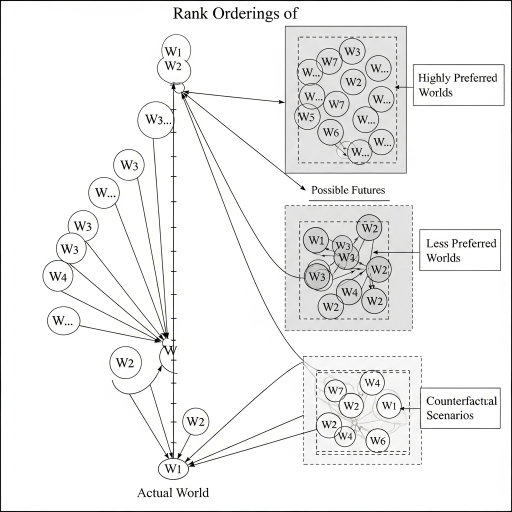
Worlds can be ranked in terms of:
probability
desirability
Learning the drivers of desirability helps determine the probability of human choice and action.
Fixing the attributes of different alternatives allows us to estimate their desirability and course of probable choice.
Revealed Preference
Utility driven Choice

“How can we learn what drives human choice?”
- Utility maximization
- Rational decision-making
- Expected value calculations
- Impulse and advertising?
Each path taken tells a story of preference and reveals something about how the attributes of each alternative tempt or repel the chooser
Relative Utility and Marginal Effects
Paths Diverge
Do you value the company of others? Do you fear it? What about the average cave dweller?
 \[ u(\text{Light shaft + Silence}) - u(\text{Glowing Fire + Conversational Echoes}) > 0?\]
PyMC-Marketing

Bayesian Marketing Analytics
- Media Mix Modelling, Customer Lifetime Value and Consumer Choice.
- Uncertainty-aware decisions: model not just what people choose, but how sure we are.
- Causal inference ready: run interventions, not just predictions.
- Modern Bayesian engine for scalability, flexibility, and transparency.
- Intuitive syntax with powerful underlying math.
Choice Data
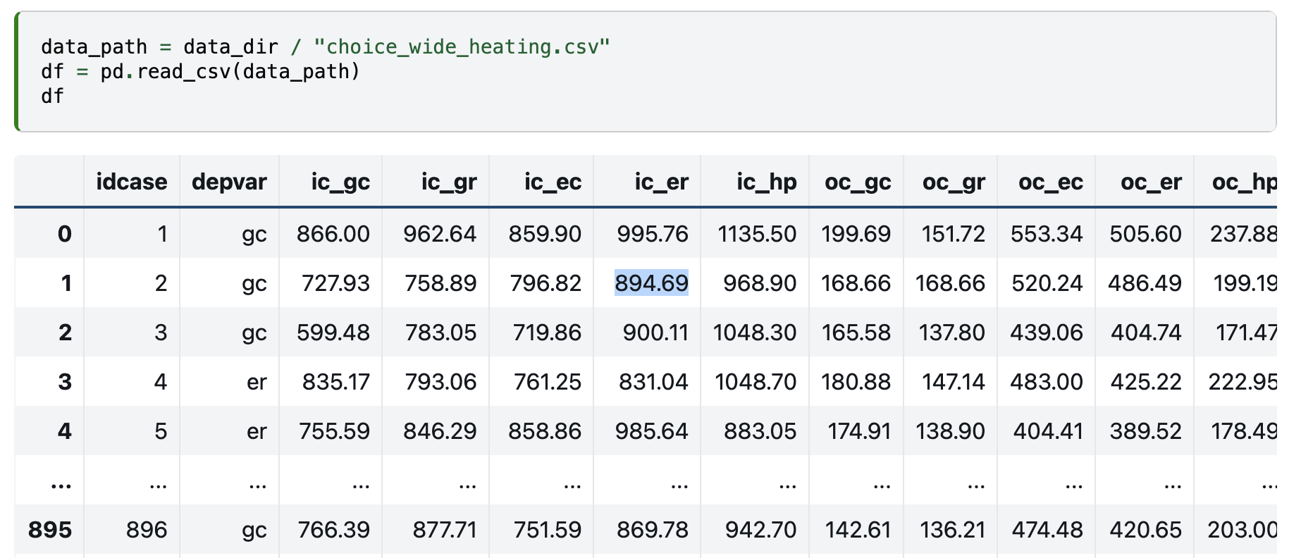
Choice Scenarios specified with attributes and choice outcomes for each discrete alternative
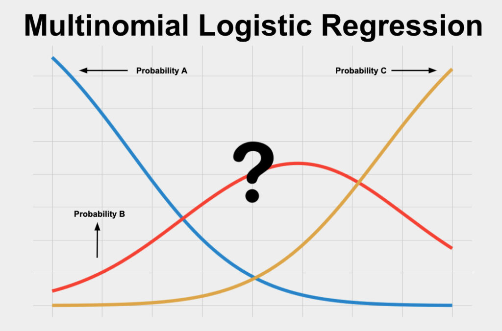
Multinomial Logit: The Simple Path Forward
The probability of choosing alternative \(j\) follows the elegant logistic form:
\[\frac{\exp(\color{red}U_{ij})}{\sum_{k=1}^{J} \exp(\color{red}U_{ik})} = P_{ij} \Rightarrow s_{j}(\color{blue}\theta_{w})=P(u_{j}>u_{k};\forall_{k̸=j})\]
A simple model with a compelling interpretation. Too simple?
PyMC-Marketing Implementation
Trace Paths through Possible Worlds
utility_formulas = [
    "gc ~ ic_gc + oc_gc | income + rooms + agehed",
    "gr ~ ic_gr + oc_gr | income + rooms + agehed",
    "ec ~ ic_ec + oc_ec | income + rooms + agehed",
    "er ~ ic_er + oc_er | income + rooms + agehed",
    "hp ~ ic_hp + oc_hp | income + rooms + agehed",
]

mnl = MNLogit(df, utility_formulas, "depvar", covariates=["ic", "oc"])
mnl.sample()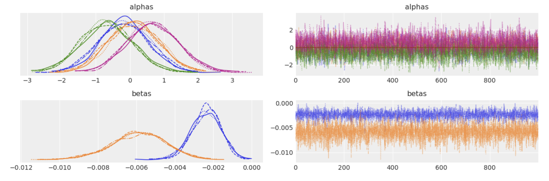
The IIA Problem - A Plot Twist

- 50% Red Bus 50% Car
- What happens if we introduce a Blue Bus?
- 33% Red Bus, 33% Blue Bus, 33% Car
The Multinomial Logit enforces the Indepdence of Irrelevant Alternatives property into preference calculations.
\[\dfrac{P_{j}}{P_{i}} = \dfrac{ \dfrac{e^{U_{j}}}{\sum_{i}^{n}e^{U_{k}}}}{\dfrac{e^{U_{i}}}{\sum_{i}^{n}e^{U_{k}}}} = \dfrac{e^{U_{j}}}{e^{U_{i}}} = e^{U_{j} - U_{k}}\]
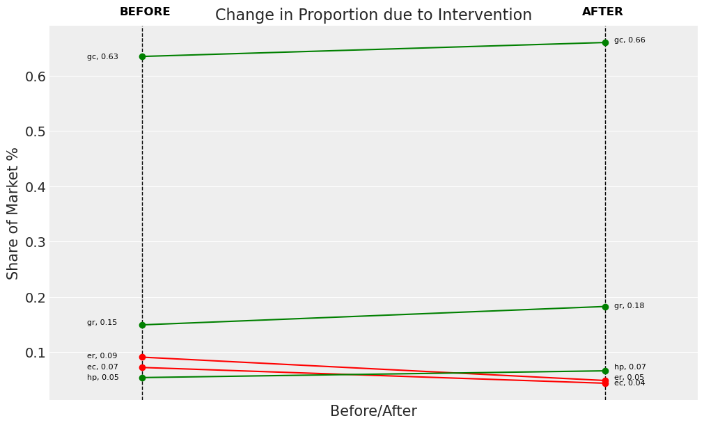
Key Take-away: The Model Ignores Market Structure
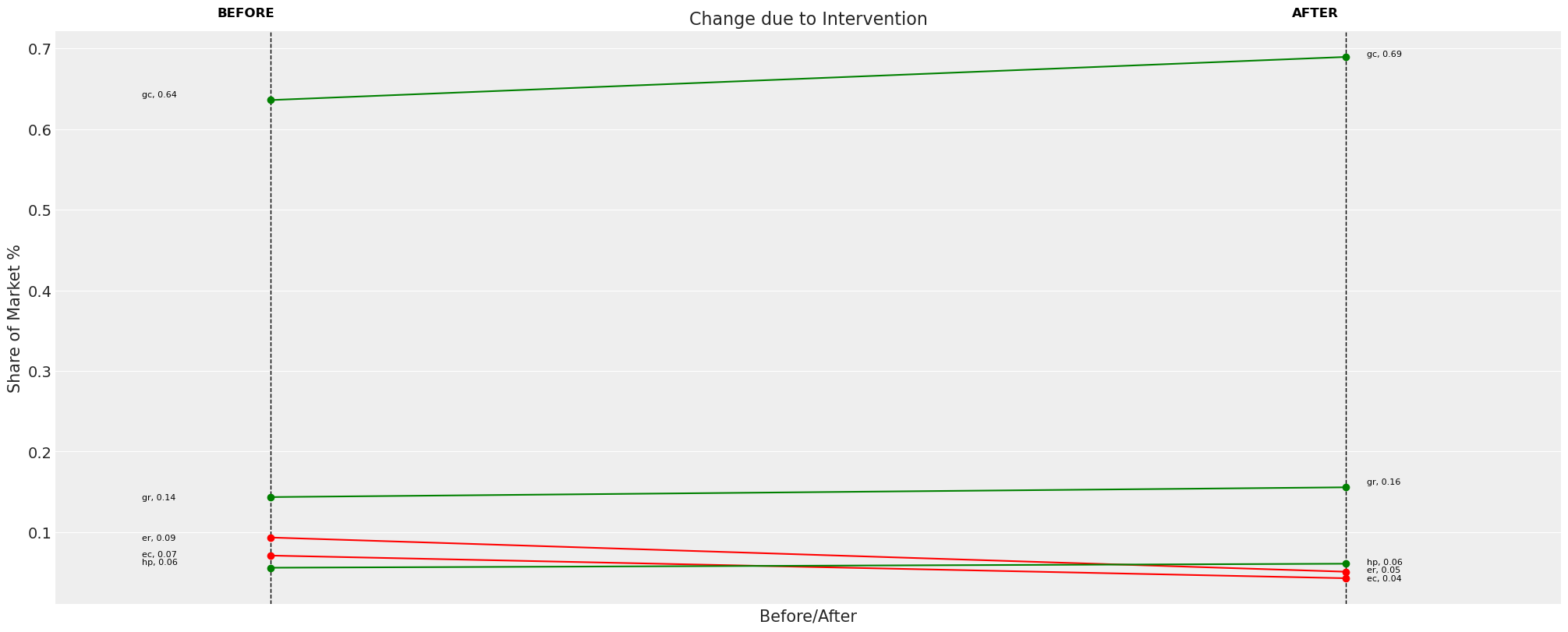
Counterfactual Inference
Counterfactual Plausibility as Criteria of Adequacy
new_policy_df = df.copy()
new_policy_df[["ic_ec", "ic_er"]] = new_policy_df[["ic_ec", "ic_er"]] * 1.5

## Posterior Predictive Forecast under counterfactual setting
idata_new_policy = mnl.apply_intervention(new_choice_df=new_policy_df)

## Compare Old and New Policy Settings
change_df = mnl.calculate_share_change(mnl.idata, mnl.intervention_idata)
change_df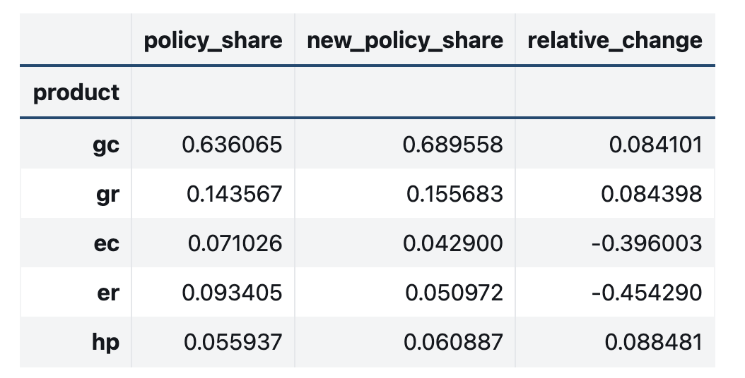
Here be Dragons

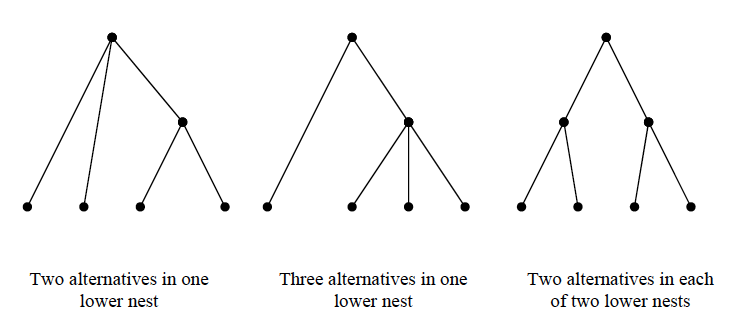
Considered Choice
Branching Probability Trees
- \(U = Y + W\)
\(P(i) \text{ when } i \in Alts\)
\(P(\text{choose nest B}) \cdot P(\text{choose i} | \text{ i} \in \text{B})\)
- \(P(\text{choose nest B}) = \dfrac{e^{W + \lambda_{k}I_{k}}}{\sum_{l=1}^{K} e^{W + \lambda_{l}I_{l}}}\)
- \(P(\text{choose i} | \text{ i} \in \text{B}) = \dfrac{e^{Y_{i} / \lambda_{k}}}{\sum_{j \in B_{k}} e^{Y_{j} / \lambda_{k}}}\)
\(I_{k} = ln \sum_{j \in B_{k}} e^{Y_{j} / \lambda_{k}} \\ \text{ and } \lambda_{k} \sim Beta(1, 1)\)
The log-sum component allows for the utility of any alternatives within a nest to “bubble up” and influence the attractiveness of the overall nest.
Behaviourial Insight in Product Preference
The relative importance of product attributes implied by our observed data
The relative importance of installation costs versus operating costs might suggest where to impose a novel pricing strategy?
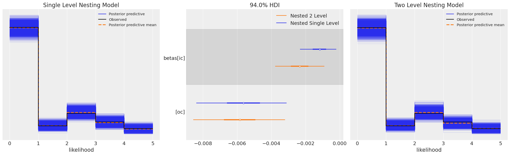
Credible Counterfactuals
Non-Proportional Substitution
new_policy_df = df.copy()
new_policy_df[["ic_ec", "ic_er"]] = new_policy_df[["ic_ec", "ic_er"]] * 1.5

idata_new_policy_1 = nstL_1.apply_intervention(new_choice_df=new_policy_df)
change_df_1 = nstL_1.calculate_share_change(nstL_1.idata, nstL_1.intervention_idata)
change_df_1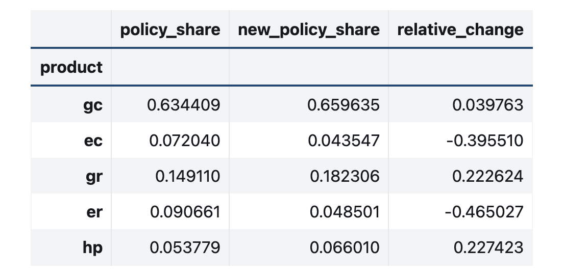
Nested Logit allows for patterns of Non-Proportional Substitution under counterfactual settings
Market Interventions and Implied Worlds
with pm.do(
    model,
    {"X1": np.ones(len(df)),
    "beta1": 0.5},
    prune_vars=True,
) as counterfactual_model:
    idata_trt = pm.sample_posterior_predictive(idata,
    var_names=["like", "p"])
Causal Inference with the Do-Operator modifies world-state and data alike allowing for compelling intervention studies about consumer behaviour
\[ w = \{ \alpha, \beta^{1}, \beta_{2}, X^{1}, X^{2} \} \\ \Rightarrow w^{*} = \{ \alpha, \beta^{*}, \beta_{2}, X^{*}, X^{2} \} \]
Conclusion: Explore the Branching Worlds
- Bayesian Models offer a data-informed tool for simulation experiments for ceteris-paribus inference.
- Plausible counterfactual inference depends on compelling world structure encoded in the model.
- Nested Logit models in PyMC-Marketing allows us to encode market structures for compelling intervention studies.
- They also reveal behaviorial insights of consumers unlocking new marketing strategies for your adventure!