Uncertainty and Causal Inference in Python
CausalPy and Quasi-Experimental Designs
Data Science @ Personio
and Open Source Contributor @ PyMC
11/16/24
The Pitch
Causal inference guides decision making. Not all questions can be answered with A/B testing. Causal impact needs to be credible anyway!
This is where you should leverage CausalPy and Bayesian causal modelling for the quantification of uncertainty and sensitivity analysis in the evaluation of policy impact.
Agenda
- Being a Data Scientist in Industry
- Causal Inference and Credibility
- Bayesian Causal Models and Design Patterns
- Complementary Practices
- IV designs
- Instrument Choice
- PS designs
- Weighting Schemes
- Conclusion: Sensitivity Analysis:
- Uncertainty in the Model
- Uncertainty about the Model
Preliminaries
Who am I?
- I’m a data scientist at Personio
- Bayesian statistician,
- Reformed philosopher and logician.
- Website: https://nathanielf.github.io/
Code or it didn’t Happen
The worked examples used here can be found here

My Website
Data Science in Industry
and other varieties of Satisficing
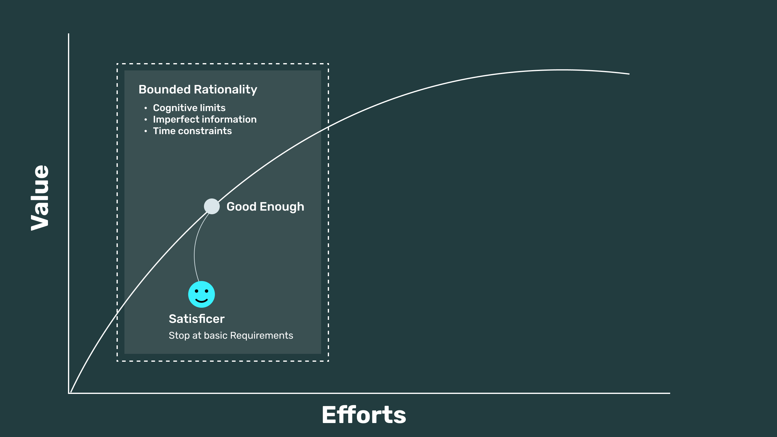
Where do we get to if everyone does the minimum? What is the compounding effect of poor decisions?
Directionally Correct …
Maybe in a ZIRP world
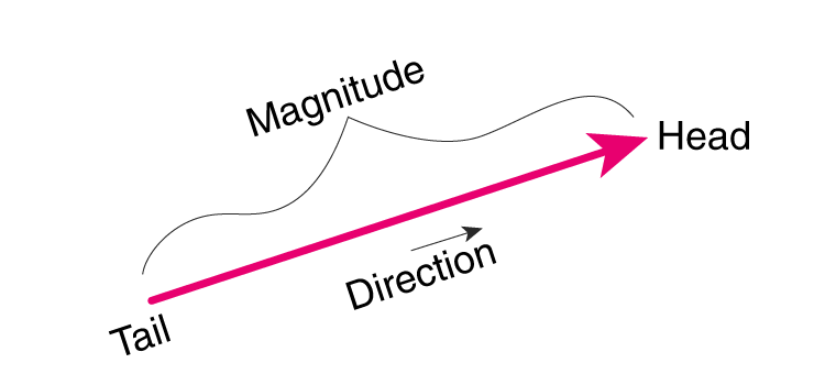
- Important investment decisions require a view of magnitude and direction.
- Most business decisions reflect some kind of investment
- But time and effort are harder to place on a balance sheet
- Only sound causal inference supports generalisable decision rules
- “Directionally Correct” is a Zero-interest-rate-phenomena.
Experiment Recipes, Rules and Responsibility
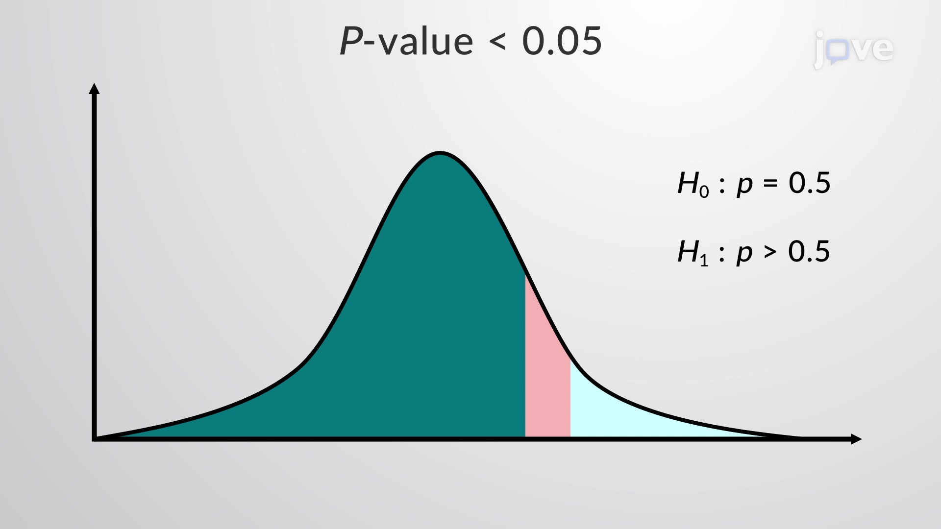

- P-value based decision criteria on policy change questions are based on the null model of an asymptotic univariate distribution.
- Most aggregate data (e.g. Total Revenue) we see in industry result from a complex array of mixture distributions and any long-run aggregates take time to converge.
- Management often doesn’t want to spend the time to validate the long-run characteristics of a phenomena that we would observe in a well powered A/B test.
- Risks underpowered experiments through a HIPPO-like decision rules and costly mistakes, ungeneralisable effects.
- Challenge: How to improve decision quality in a resource constrained/time-bound environment?
Causal Inference, Crediblility
… and Quasi-Experimental Design
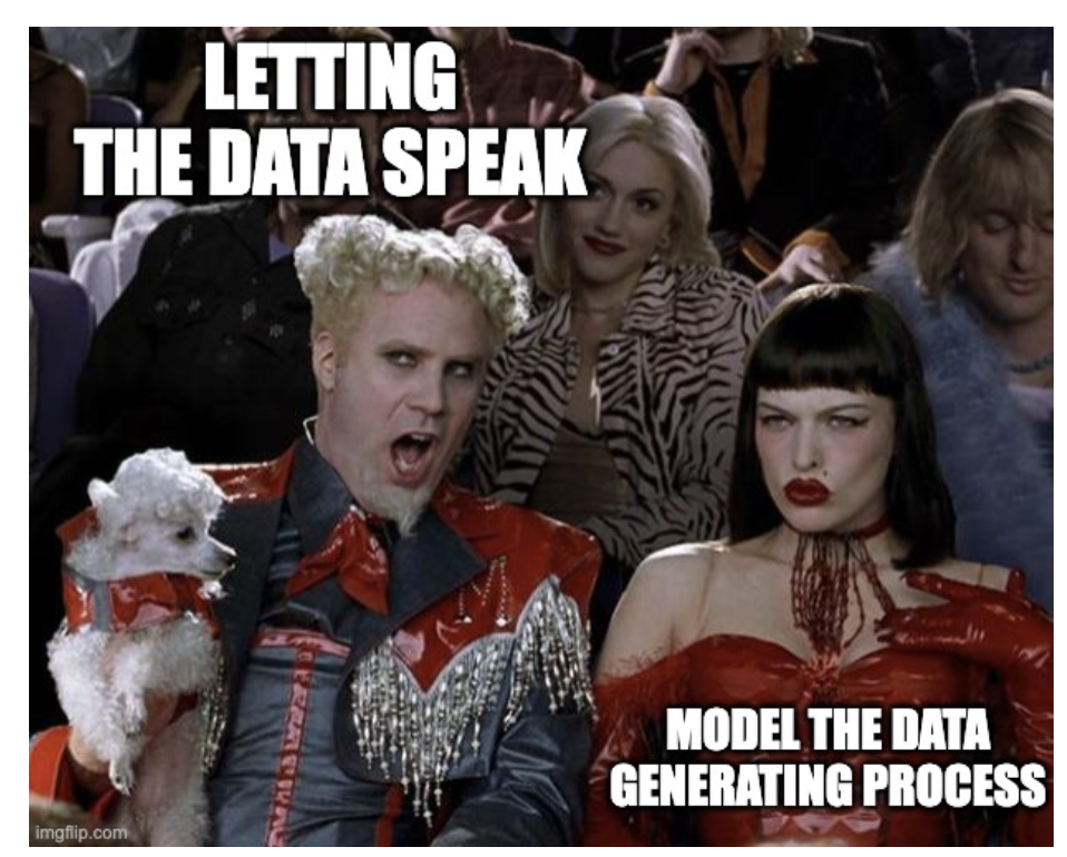
- If the data can speak for itself, the answer is usually blindingly obvious or has taken an inordinate amount of time to accumulate
- More generally, if we’ve modeled the data generating process we can answer an array of subtle questions about cause and effect that support effective decision-making.
- Approach: Communicate and pursue opportunities for natural experiments. Build credibility through linking theoretical estimand and empirical data while partnering across the business with subject matter experts.
CausalPy and Bayesian Inference

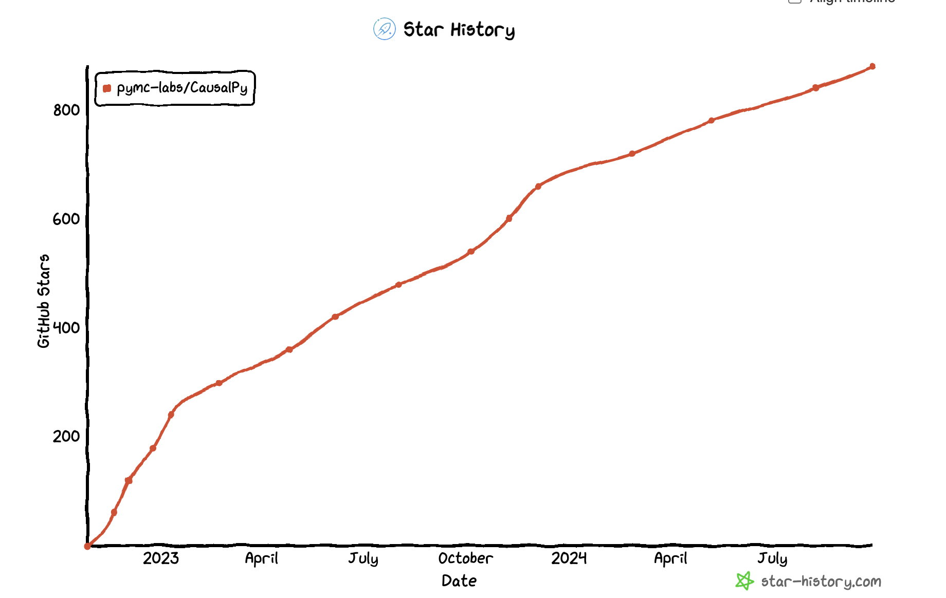
- A python package for Bayesian Models and Causal Inference methods
- Developed and maintained by @PyMC Labs
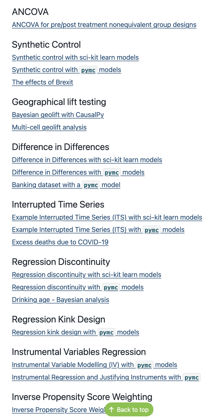
- Broad Coverage of quasi-experimental designs.
Causal Methods and Models
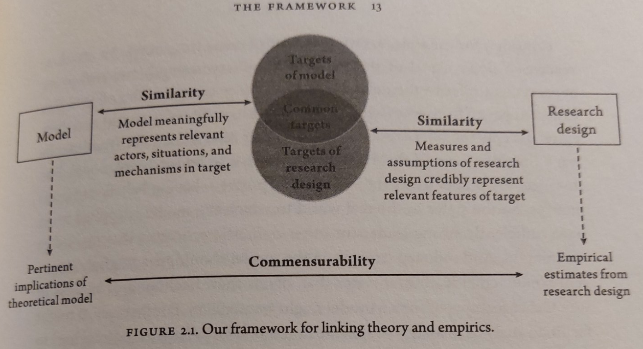 Causal question(s) of import can be interrogated just when we can pair a research design with an appropriate statistical model.
Canonical DAGs and Methods
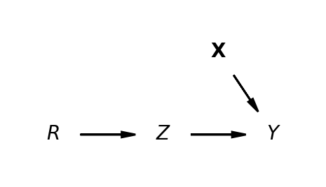
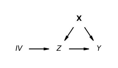
The treatment effect can be estimated cleanly \[ y \sim 1 + Z \]
The treatment effect has to be estimated so as to avoid the bias due to X \[ y \sim 1 + \widehat{Z} \] \[ \hat{Z} \sim 1 + IV \]
IV Regression in CausalPy
N = 100
e1 = np.random.normal(0, 3, N)
e2 = np.random.normal(0, 1, N)
Z = np.random.uniform(0, 1, N)
## Ensure the endogeneity of the the treatment variable
X = -1 + 4 * Z + e2 + 2 * e1
y = 2 + 3 * X + 3 * e1

test_data = pd.DataFrame({"y": y, "X": X, "Z": Z})

sample_kwargs = {
    "tune": 1000,
    "draws": 2000,
    "chains": 4,
    "cores": 4,
    "target_accept": 0.99,
}
instruments_formula = "X  ~ 1 + Z"
formula = "y ~  1 + X"
instruments_data = test_data[["X", "Z"]]
data = test_data[["y", "X"]]
iv = InstrumentalVariable(
    instruments_data=instruments_data,
    data=data,
    instruments_formula=instruments_formula,
    formula=formula,
    model=InstrumentalVariableRegression(sample_kwargs=sample_kwargs),
)
Bayesian Structural Model
And Instrument Strength
\[\begin{align*} \left( \begin{array}{cc} Y \\ Z \end{array} \right) & \sim \text{MultiNormal}(\color{green} \mu, \color{purple} \Sigma) \\ \color{green} \mu & = \left( \begin{array}{cc} \mu_{y} \\ \mu_{z} \end{array} \right) = \left( \begin{array}{cc} \beta_{00} + \color{blue} \beta_{01}Z ... \\ \beta_{10} + \beta_{11}IV ... \end{array} \right) \end{align*} \]
The treatment effect \(\color{blue}\beta_{01}\) of is the primary quantity of interest
\[ \color{purple} \Sigma = \begin{bmatrix} 1 & \color{blue} \sigma \\ \color{blue} \sigma & 1 \end{bmatrix} \]
The Bayesian estimation strategy incorporates two structural equations and the success of the IV model relies of the correlation between terms.
Returns to Schooling: Concrete Example
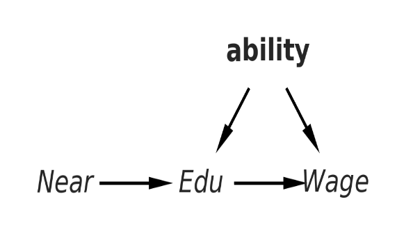
Recipe of Assumptions:
- Exclusion Restriction
- Independence
- Relevance
Returns to Schooling: Instrument Relevance
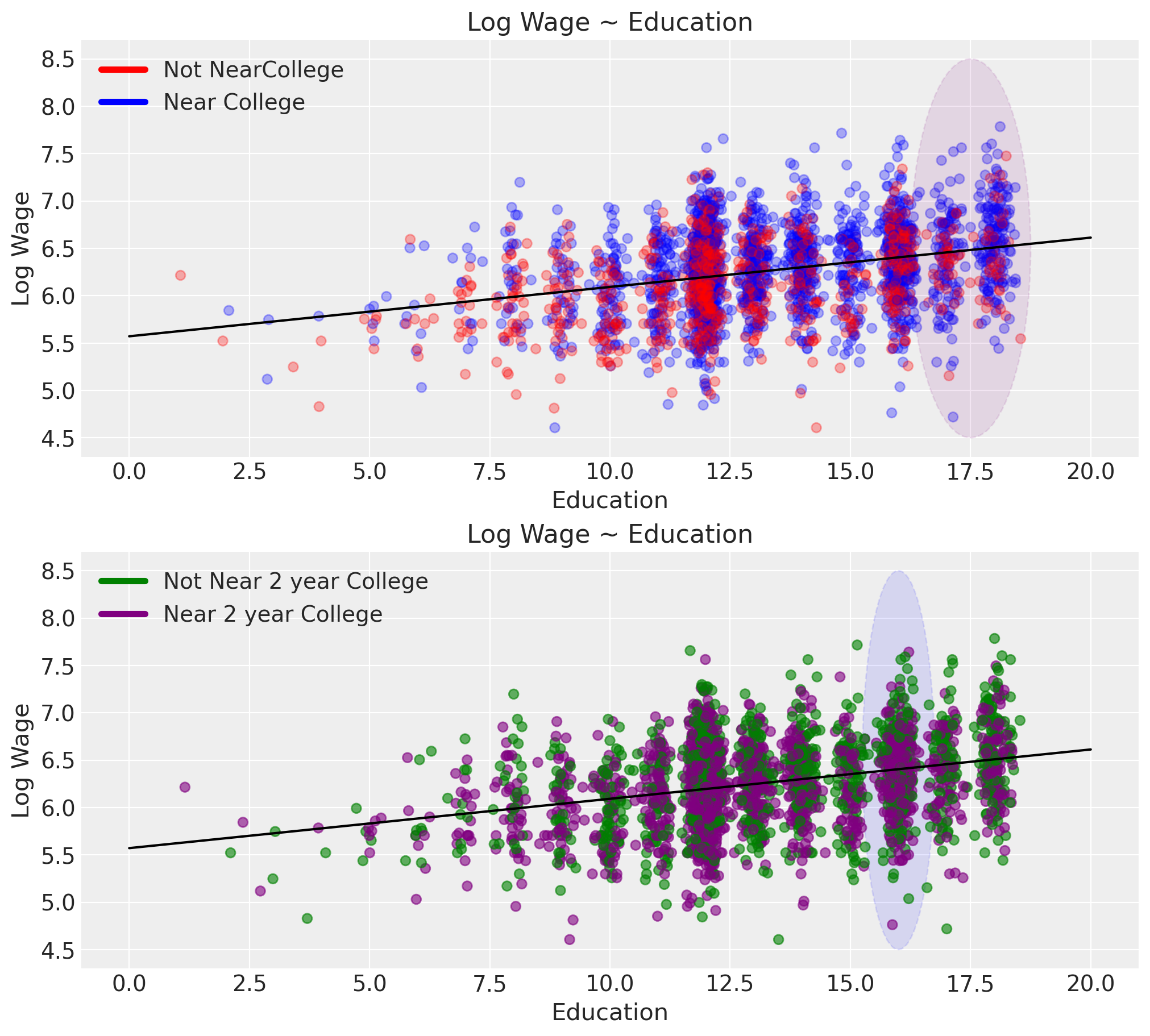
We want to argue for:
the relevance of our instrument i.e. that it has a non-trivial impact on the outcome of interest
that it influences the result only via the treatment condition.
evaluating multiple instrument candidates
Returns to Schooling: Quantifying Confounding
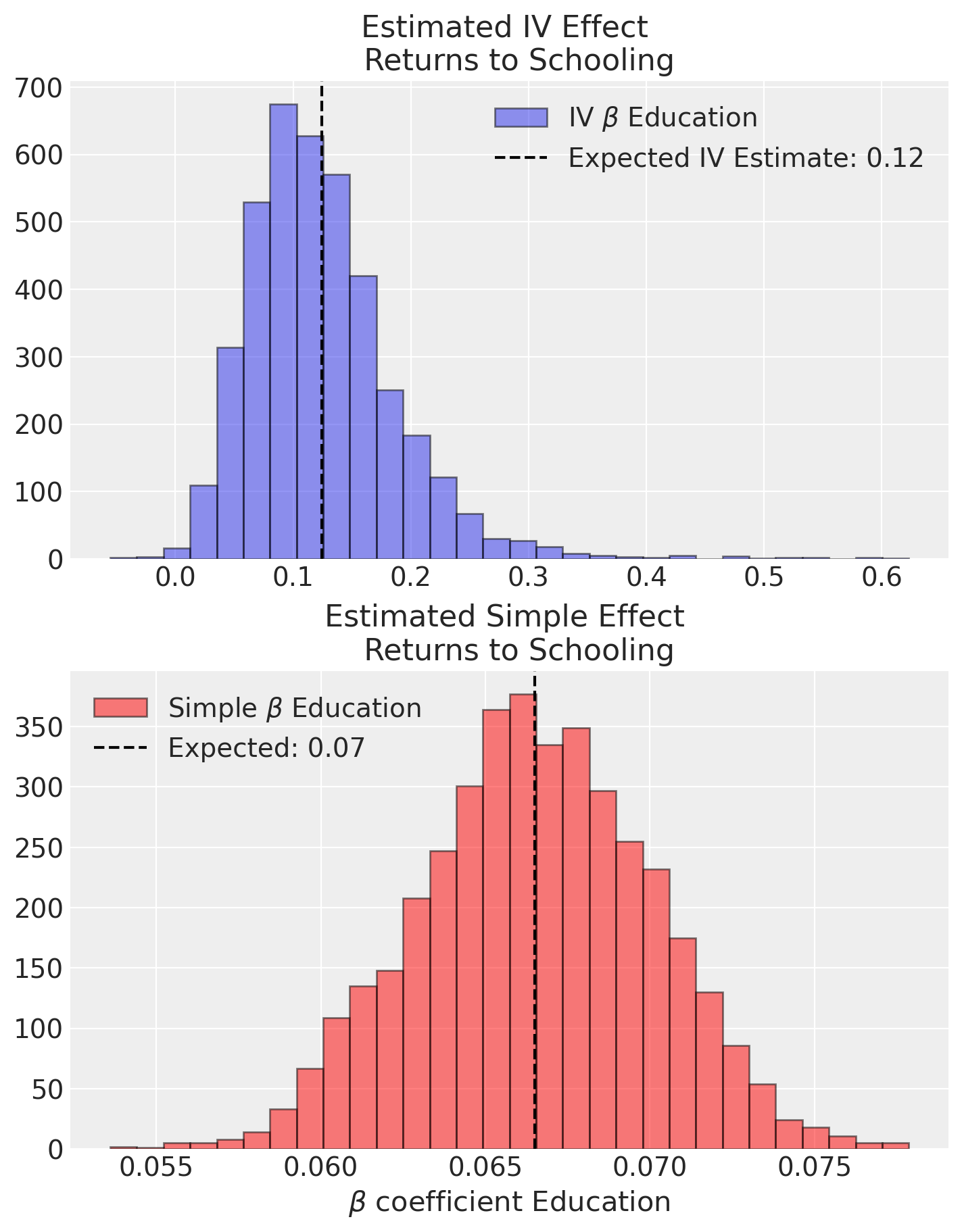
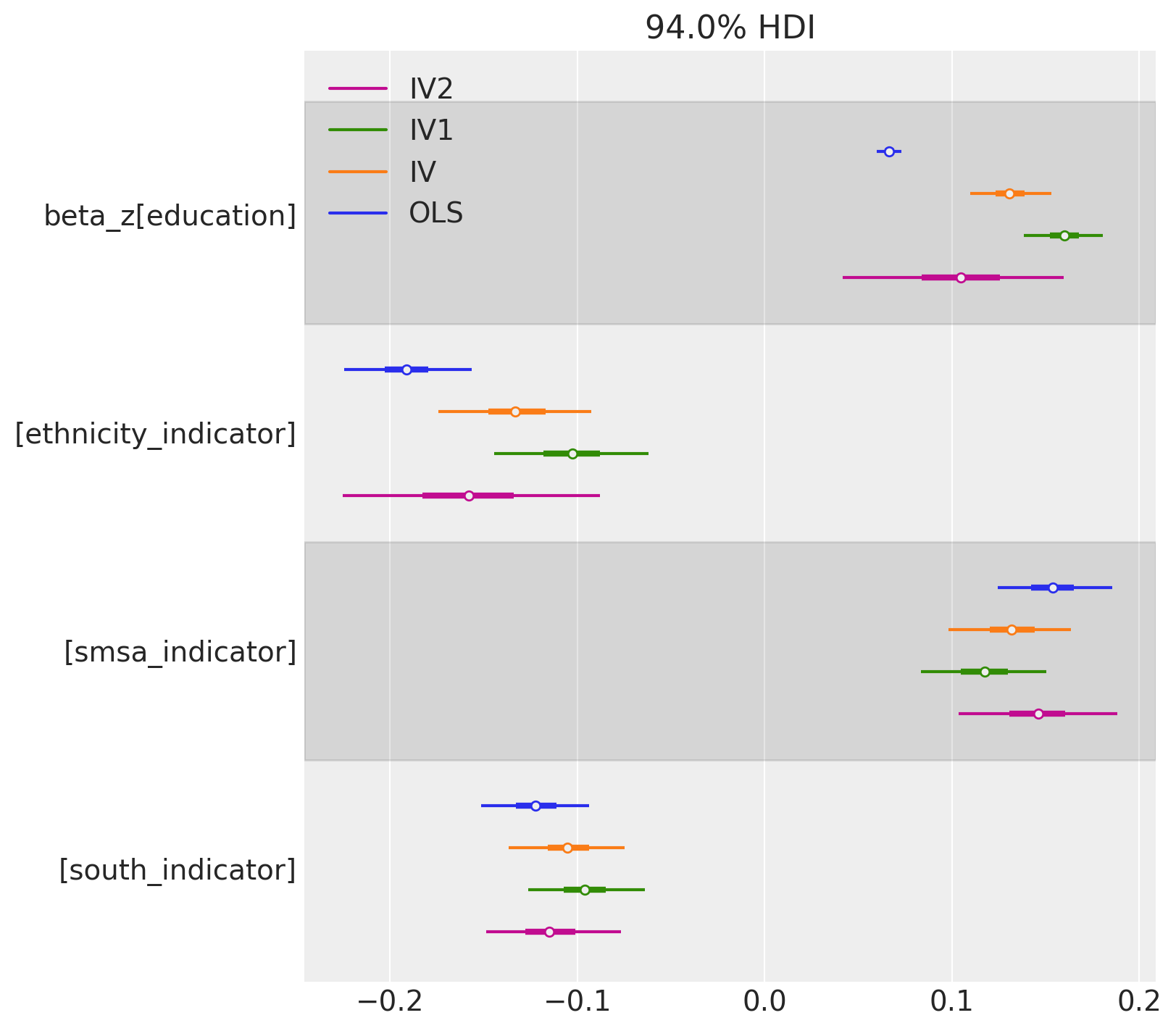
The natural comparison with OLS shows:
evidence of genuine confounding in the estimates of treatment effect
Crucially it highlights the false precision in the OLS estimate.
Model comparison is at the heart of understanding confounding in causal infernece.
IV models may be compared by structure but also by instruments used.
Returns to Schooling: Justifying Instruments
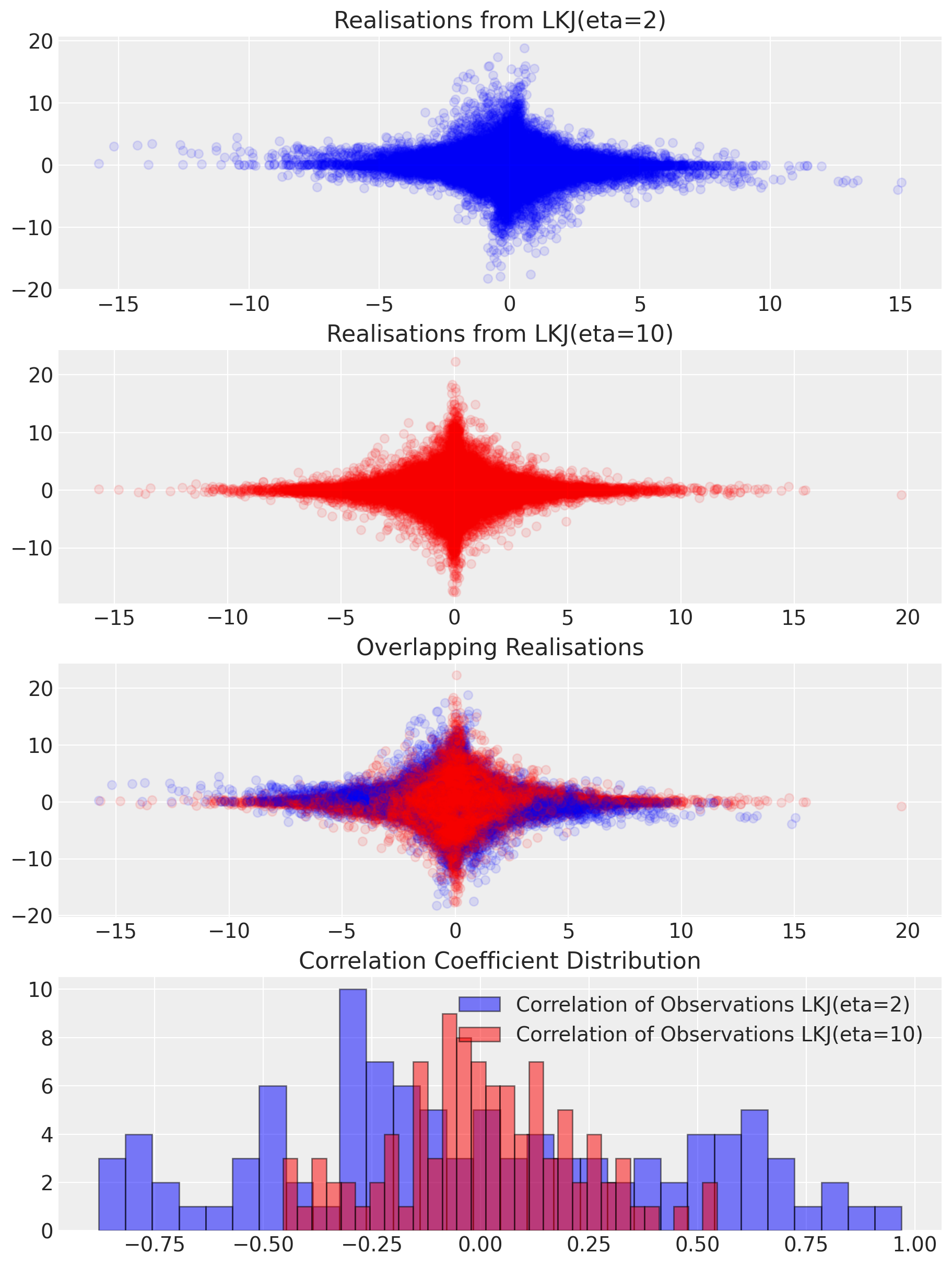
The strength of an instrument is determined by the correlation structure between instrument and outcome via the treatment solely:
F-tests can be used to assess how the instrument relates to the outcome.
In the Bayesian setting we can directly estimate the correlation structure and apply sensitivity tests.
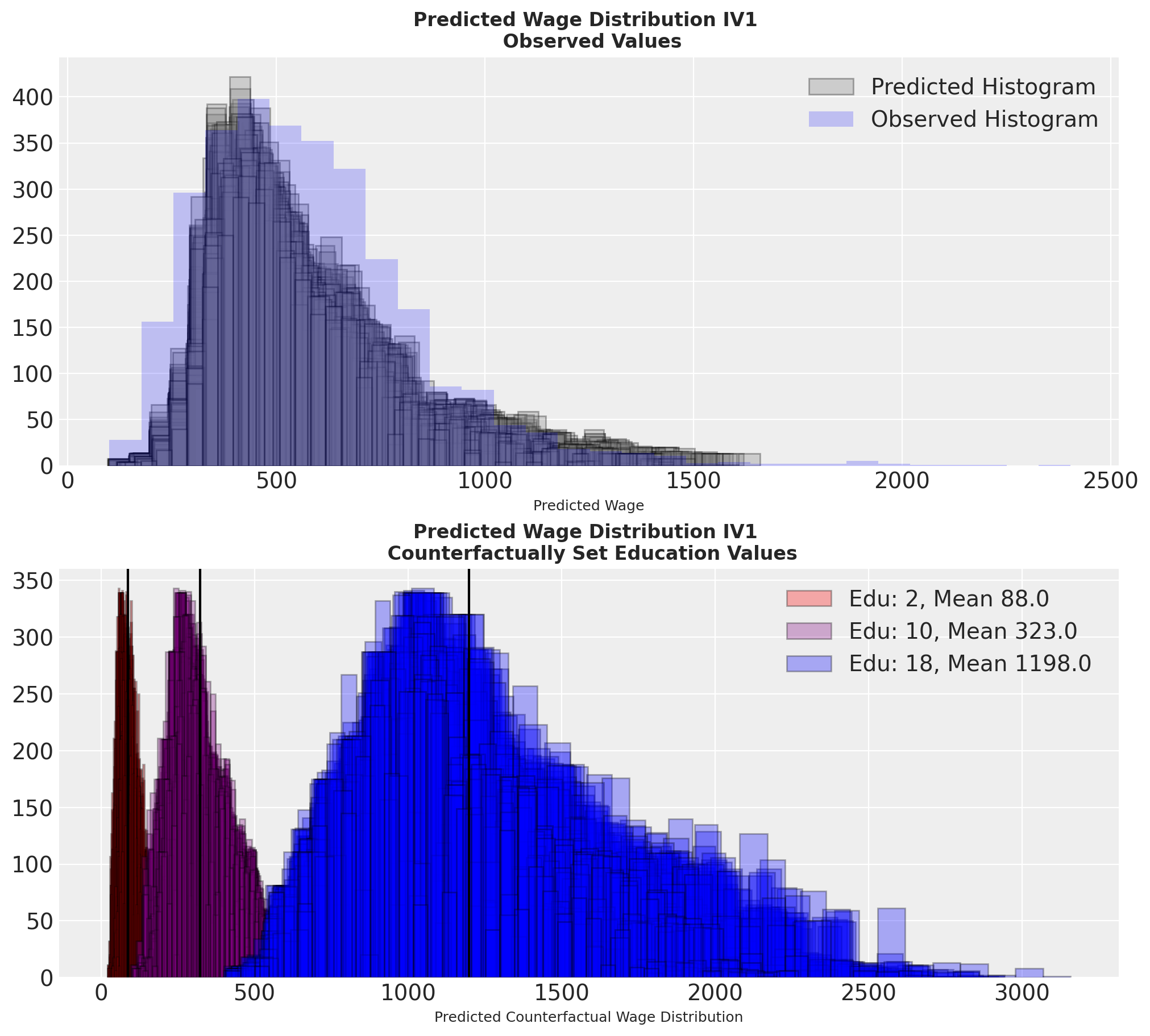
Stronger priors on correlation strength influence the outcomes and can be evaluated against the data through posterior predictive checks
Returns to Schooling: Sensitivity Analysis and Model Evaluation
Canonical DAGs and Methods


The treatment effect can be estimated cleanly \[ y \sim 1 + Z + X_1 ... X_N \] \[ p(Z) \sim X_1 ... X_N \]
Propensity score adjustments reweight our outcome by the probability of treatment \[ y \sim f(p(Z), Z)\]
Propensity Scores in CausalPy
df1 = pd.DataFrame(
    np.random.multivariate_normal([0.5, 1], [[2, 1], [1, 1]], size=10000),
    columns=["x1", "x2"],
)
df1["trt"] = np.where(
    -0.5 + 0.25 * df1["x1"] + 0.75 * df1["x2"] + np.random.normal(0, 1, size=10000) > 0,
    1,
    0,
)
TREATMENT_EFFECT = 2
df1["outcome"] = (
    TREATMENT_EFFECT * df1["trt"]
    + df1["x1"]
    + df1["x2"]
    + np.random.normal(0, 1, size=10000)
)

result1 = cp.InversePropensityWeighting(
    df1,
    formula="trt ~ 1 + x1 + x2",
    outcome_variable="outcome",
    weighting_scheme="robust",
    model=cp.pymc_models.PropensityScore(
        sample_kwargs={
            "draws": 1000,
            "target_accept": 0.95,
            "random_seed": seed,
            "progressbar": False,
        },
    ),
)

result1
Propensity Score Models
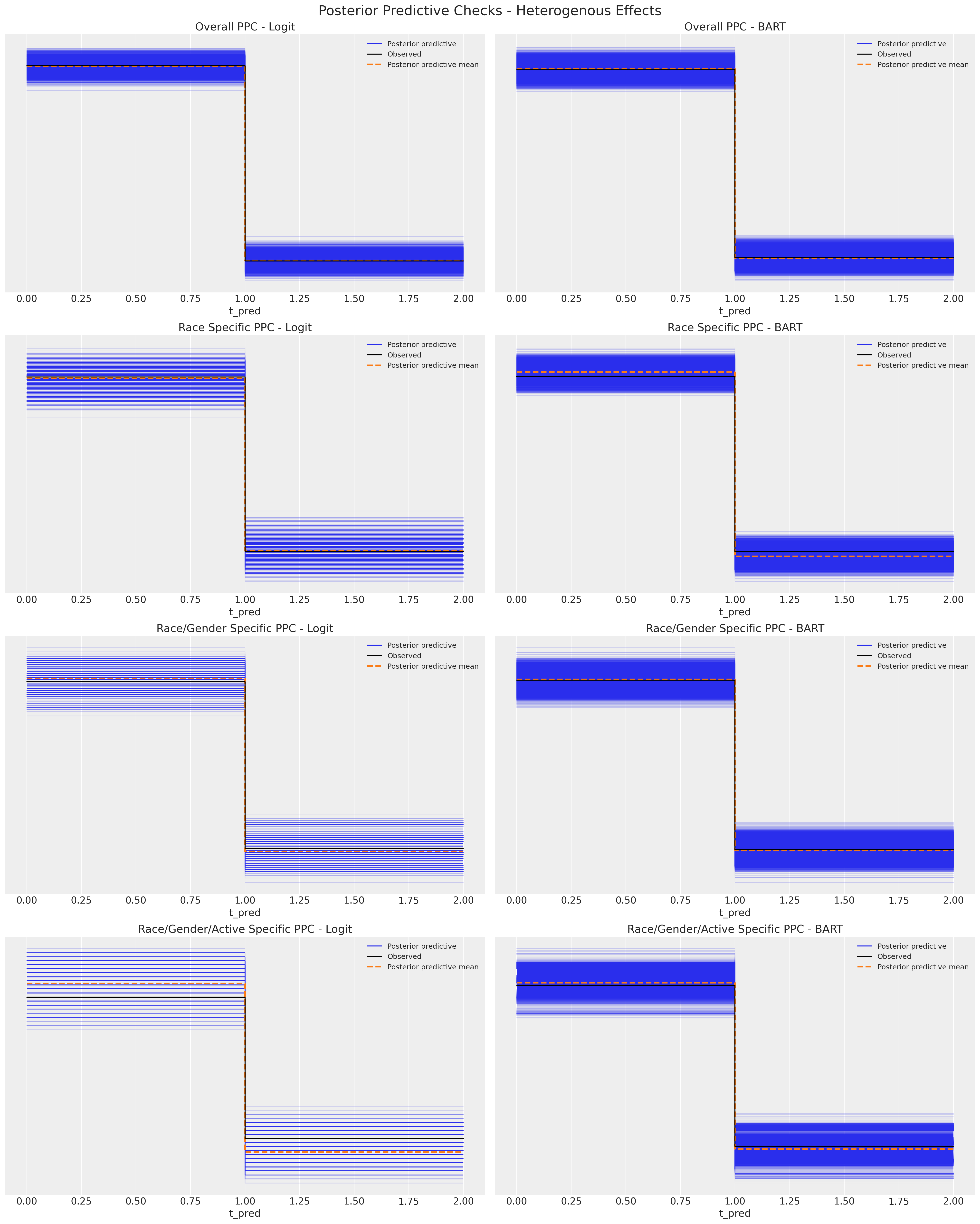
Overfitting Propensity Score models to the sample data confounds causal inference
Validating Balancing Effects

Balancing Covariate Distributions across Treatment Groups
Balanced covariate distributions is testable implication the propensity score design.
Models and Weighting Methods
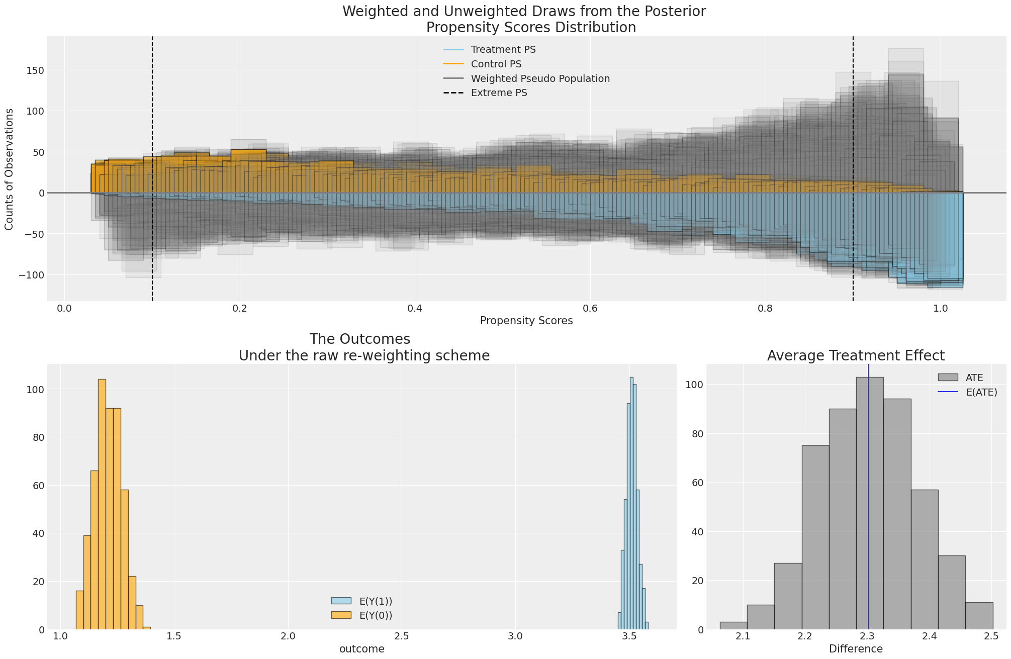
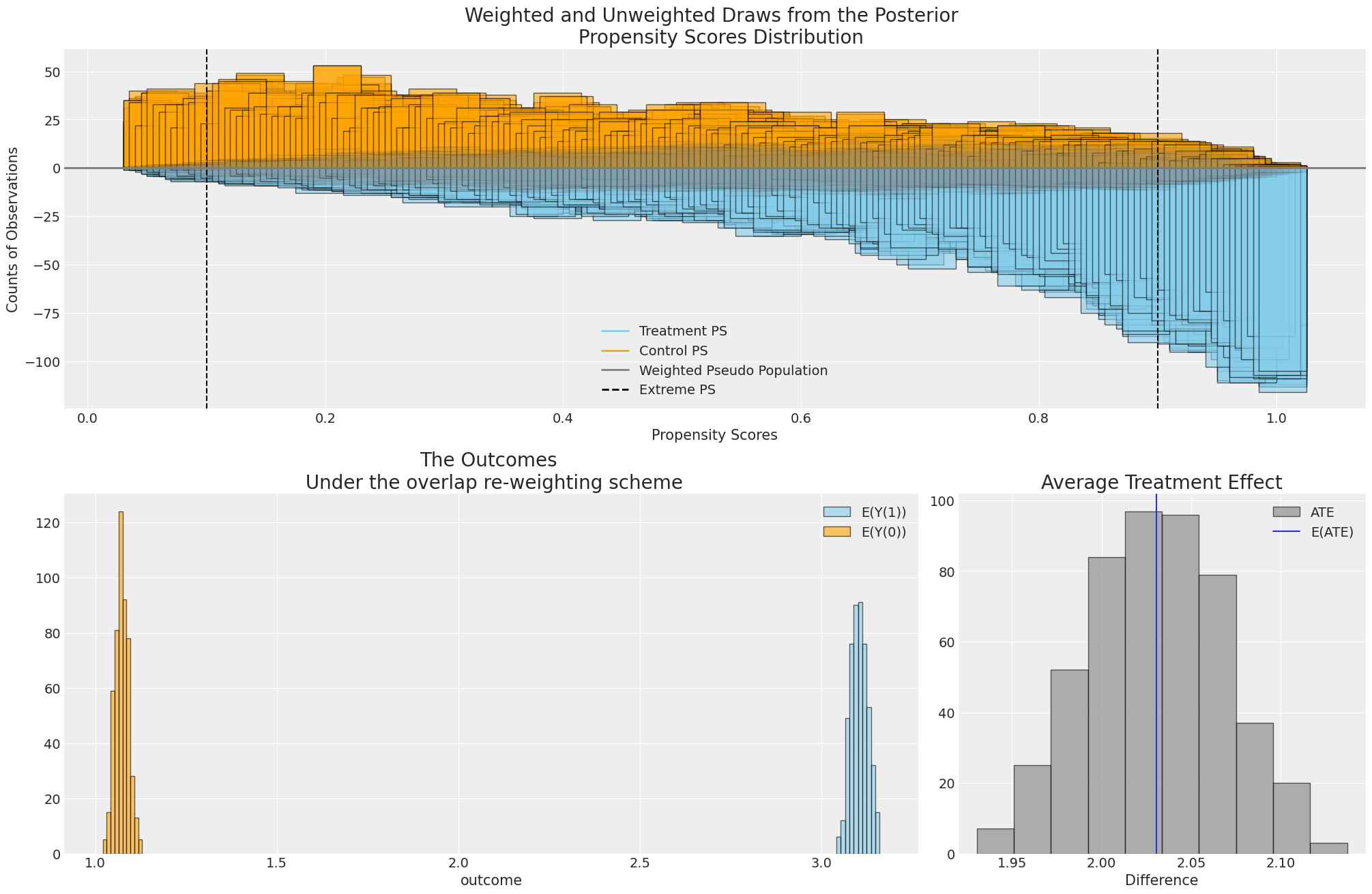
Propensity Weighting Adjusts Outcome Distribution to improve estimation of treatment effects
Conclusion
- Uncertainty in the Model
- Causal inference wrestles with the uncertain consequence(s) of assumed data generating processes.
- Bayesian Causal Inference takes uncertainty quantification seriously
- Prior sensitivity Analysis further establishes the robustness of our estimates under uncertainty
- Uncertainty about the Model
- The combinatorial complexity of the possible models necessitates informed opinion to zero-in on plausible models
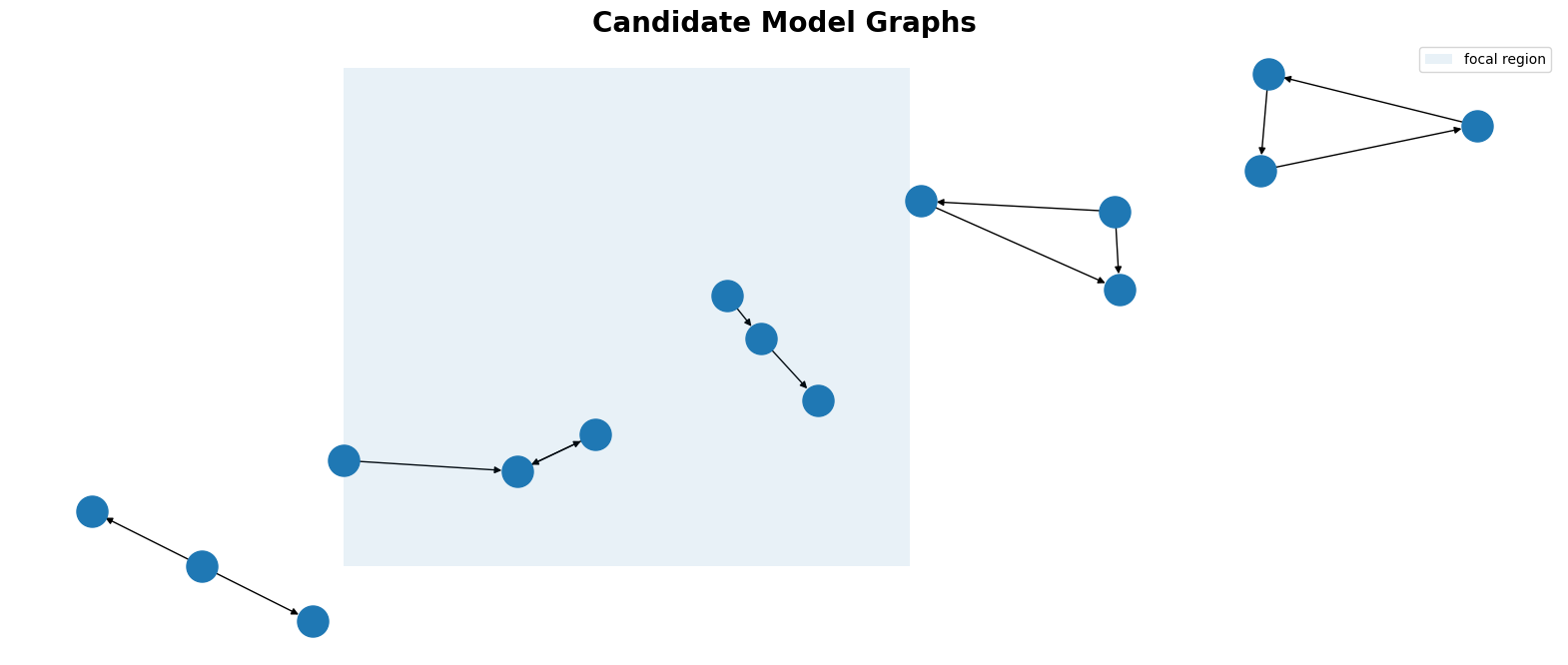
CausalPy streamlines the deployment and analysis of these causal inference models with proper tools to asses their uncertainty, and communicate impact of policy changes.
Faciliates model evaluation, comparison and combination - to build credible patterns of inference and justified approaches to critical decisions.
Causal Inference in Python