Bayesian Workflow with SEMs

PyCon Ireland 2025

Nathaniel Forde

Data Science @ Personio

and Open Source Contributor @ PyMC

2025-11-16

Preliminaries

Who am I?

I’m a data scientist at Personio
- Bayesian statistician,
- Reformed philosopher and logician.
Website: https://nathanielf.github.io/

Code or it didn’t Happen

The worked examples used here can be found here

My Website

The Pitch

Structuring Your Work with Structural Equation Models

Probabilistic programming languages (PPLs) are structures for articulating assumptions and relationships, and a scaffold for exploring uncertainty.

Structural Equation models (SEMs) formalize scientific theory as a system of statistical relationships.

The Bayesian workflow binds these together into a compelling practice: an iterative conversation between theory and data disciplined by rigours of probabilistic programming

Agenda

The Idea of a Workflow:
- Craft versus Checklist
- Job Satisfaction
Bayesian Workflow with SEMs:
- Confirmatory Factor Structures
- Adding Structural Relations
- Adding Covariance Structure
Sensitivity Analysis:
- Adding Hierarchical Structure
- Parameter Recovery and Model Validation
Conclusion
- Craft and Statistical Workflow

The Idea of a Workflow

Craft in Statistical Modelling

Embraces process, imperfection, and iteration.

Aims at the acquisition of scientific knowledge

Supports generalisable findings and solutions

Restore ownership: you shape, test, and refine — the model carries your imprint.

Checklists in Statistical Modelling

Reduce inquiry to compliance: ticking boxes replaces genuine understanding.

Create the illusion of rigor while bypassing uncertainty and context.

Confuse progress with throughput: more boxes checked ≠ better science.

Promotes shallow levels of engagement, infantalises the management class. Hinders effective decision making.

Strips away ownership: you don’t make something, you just complete a task.

Job Satisfaction Data

Constructive Thought Strategies (CTS): Thought patterns that are positive or helpful, such as:
- Self-Talk (positive internal dialogue): ST
- Mental Imagery (visualizing successful performance or outcomes): MI
- Evaluating Beliefs & Assumptions (i.e. critically assessing one’s internal assumption: EBA
Dysfunctional Thought Processes: (DA1–DA3)
Subjective Well Being: (UF1, UF2, FOR)
Job Satisfaction: (JW1–JW3)

Contemporary Bayesian Workflow

Start with Theory and Prior Knowledge
Iterate with Checks and Visual Diagnostics
Refine Structure and Layer Complexity
- Assess consistency of Signal
Validate through Sensitivty Analysis
Own the Process

Structural Equation Models

Richly Parameterised Regressions with Expressive Encodings of Measurement Error and Latent Constructs

The SEM workflow

Start with Confirmatory Factor Analysis (CFA):
- Validate that our measurement model holds.
- Ensure latent constructs are reliably represented by observed indicators.

Layer Structural Paths:
- Add theoretically-motivated regressions between constructs.
- Assess whether hypothesized relationships improve model fit.

Refine with Residual Covariances:
- Account for specific shared variance not captured by factors.
- Keep structure transparent while improving realism.

Iterative Validation:
- Each step asks: Does this addition honor theory? Improve fit?
- Workflow = constant negotiation between parsimony and fidelity.

Job Satisfaction Data

	JW1	JW2	JW3	UF1	UF2	FOR	DA1	DA2	DA3	EBA	ST	MI
0	-1.046719	-1.472334	-1.649844	-0.740886	-0.573890	-0.992347	1.269461	1.805128	1.230402	-0.039732	1.618562	-0.169659
1	-1.649857	-1.908889	-1.841327	0.120929	-0.939917	0.401440	0.177058	0.126041	-0.004604	-0.806541	0.930899	-0.438887
2	0.429099	1.826533	0.341107	1.033988	1.287623	0.490457	-0.627370	-0.717461	-0.246633	0.261212	0.913639	0.496846
3	0.257582	-0.315831	1.258474	0.241065	-0.548987	-0.247273	0.858847	0.964730	1.233870	-0.251100	0.466743	0.169622
4	-0.875969	-0.263046	-0.947966	-0.231731	-0.850588	0.860900	0.989963	0.671778	0.438236	-0.129382	2.266723	-0.951899

The Data for SEM modelling is a multivariate data structure with natural theory-driven categories of variables which reflect some mis-measured latent factor.

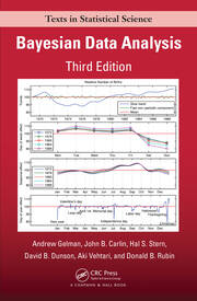
The Confirmatory Factor Structure

Bayesian Workflow with SEMs

CFA

with pm.Model(coords=coords) as cfa_model_v1:
    
    # --- Factor loadings ---
    lambdas_1 = make_lambda('indicators_1', 'lambdas1', priors=[1, .5])
    lambdas_2 = make_lambda('indicators_2', 'lambdas2', priors=[1, .5])
    lambdas_3 = make_lambda('indicators_3', 'lambdas3', priors=[1, .5])
    lambdas_4 = make_lambda('indicators_4', 'lambdas4', priors=[1, .5])

    Lambda = pt.zeros((12, 4))
    Lambda = pt.set_subtensor(Lambda[0:3, 0], lambdas_1)
    Lambda = pt.set_subtensor(Lambda[3:6, 1], lambdas_2)
    Lambda = pt.set_subtensor(Lambda[6:9, 2], lambdas_3)
    Lambda = pt.set_subtensor(Lambda[9:12, 3], lambdas_4)
    Lambda = pm.Deterministic('Lambda', Lambda)

    sd_dist = pm.Exponential.dist(1.0, shape=4)
    chol, _, _ = pm.LKJCholeskyCov("chol_cov", n=4, eta=2, sd_dist=sd_dist, compute_corr=True)
    eta = pm.MvNormal("eta", 0, chol=chol, dims=("obs", "latent"))

    # Construct Pseudo Observation matrix based on Factor Loadings
    mu = pt.dot(eta, Lambda.T)  # (n_obs, n_indicators)

    ## Error Terms
    Psi = pm.InverseGamma("Psi", 5, 10, dims="indicators")
    _ = pm.Normal('likelihood', mu=mu, sigma=Psi, observed=observed_data)

\[ \eta \sim MvN(0, \Sigma)\] \[ \mu = \color{blue}{\Lambda} \eta\] \[\mathbf{y} = N(\mu, \Psi)\]

Bayesian Workflow with SEMs

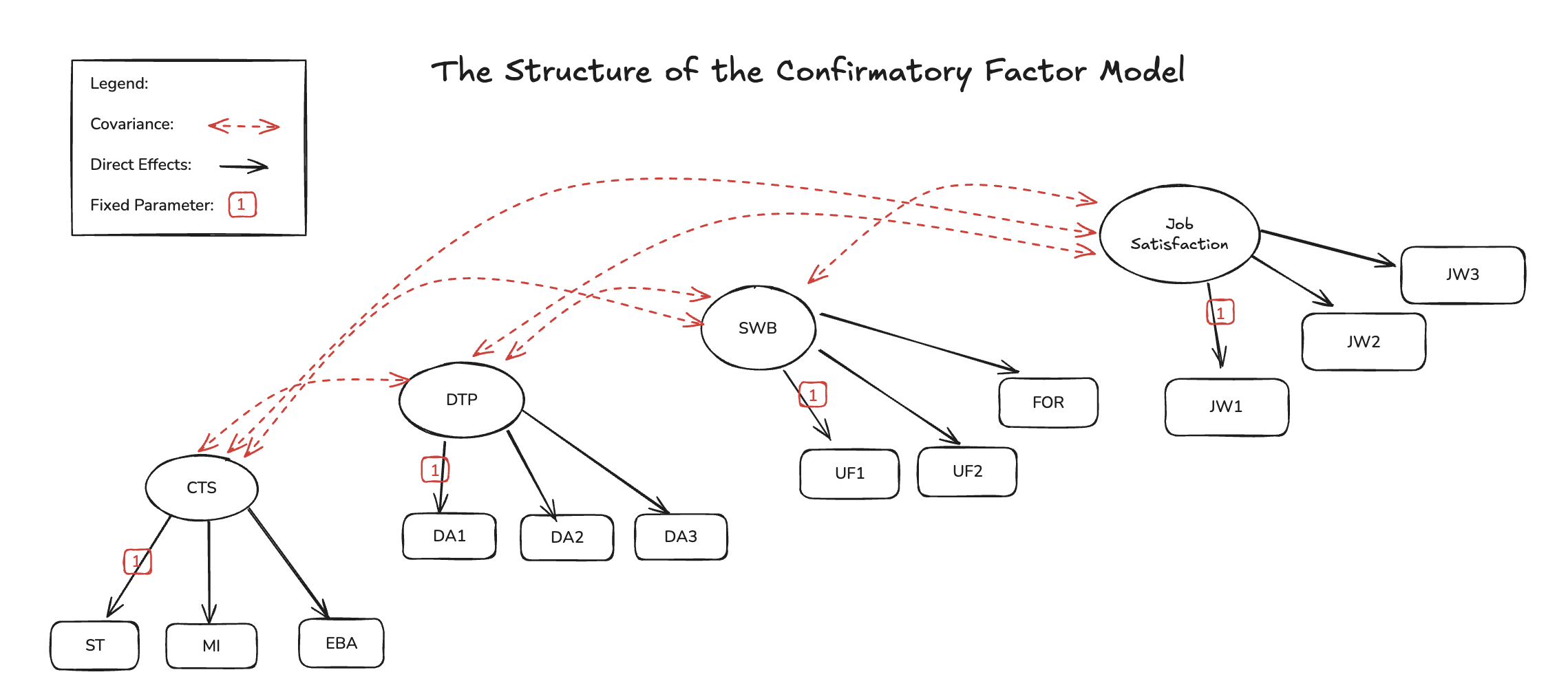
CFA Implications

Estimated Factor Loadings are close to 1
The indicator(s) are strongly reflective of the latent factor.
Posterior Predictive Residuals are close to 0
Latent factors move together in intuitive ways.
High Satisfaction ~~ High Well Being

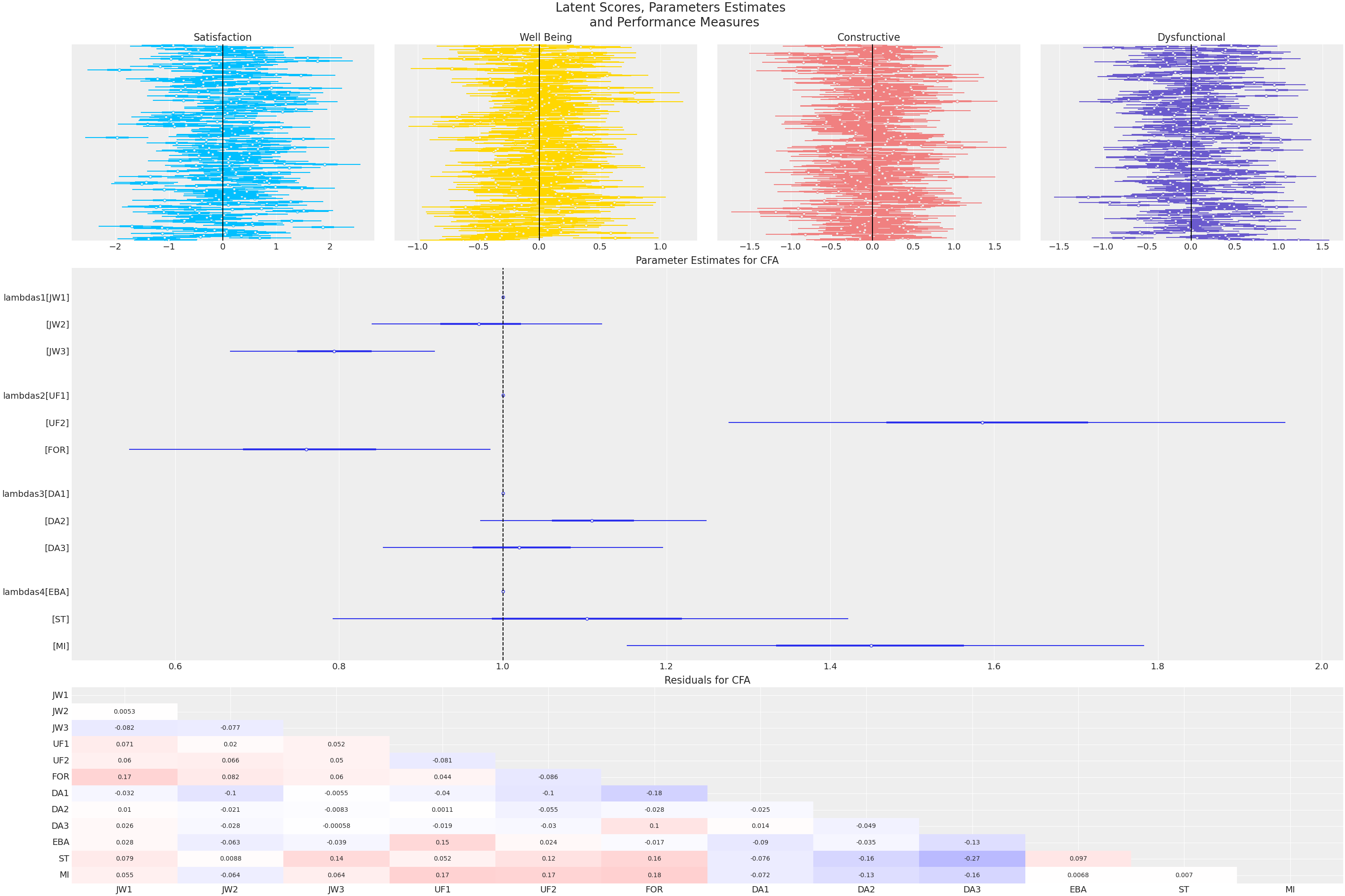
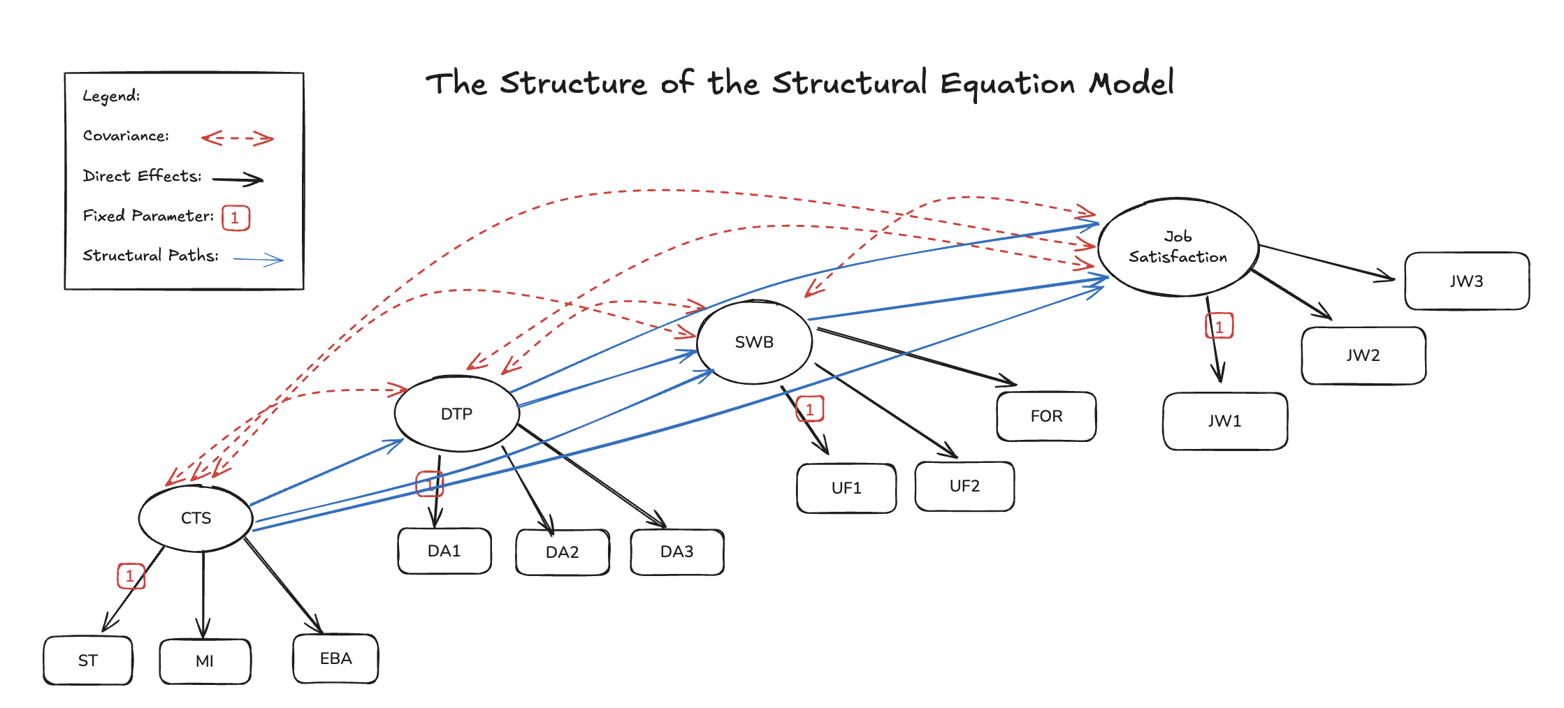
The SEM Regression

The Structural Matrix

\[ \mathbf{\gamma} = \begin{bmatrix} \overbrace{0.5}^{sat} & \overbrace{0.2}^{well being} & \overbrace{-0.3}^{dys} & \overbrace{0.7}^{con} \\ ... & ... & ... & .. \\ ... & ... & ... & .. \\ ... & ... \\ 0.4 & ...\end{bmatrix},\mathbf{B} = \begin{bmatrix} \overbrace{0}^{sat} & 0 & 0 & \overbrace{0}^{con} \\ \beta_{21} & 0 & 0 & 0 \\ \beta_{31} & \beta_{32} & 0 & 0 \\ \beta_{41} & \beta_{42} & \beta_{43} & 0 \end{bmatrix} \]

The SEM Regression

The Structural Matrix

\[ \eta = solve(I - \mathbf{B}, \mathbf{\gamma})\]

\[ \mathbf{\eta} = \begin{bmatrix} \overbrace{3.2}^{sat} & \overbrace{1.3}^{well being} & \overbrace{2.1}^{dys} & \overbrace{4.9}^{con} \\ ... & ... & ... & .. \\ ... & ... & ... & .. \\ ... & ... \\ 5.0 & ...\end{bmatrix} \]

The SEM Regression

with Mediation Effects

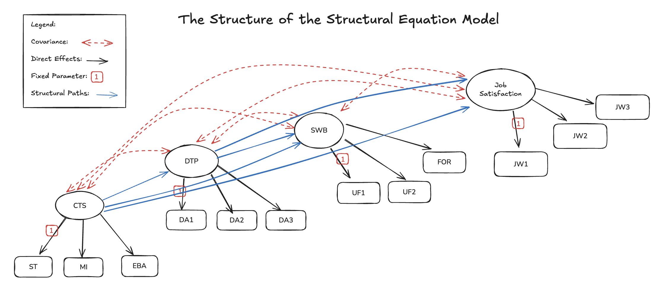
The SEM Regression

with Staggered Mediation Effects

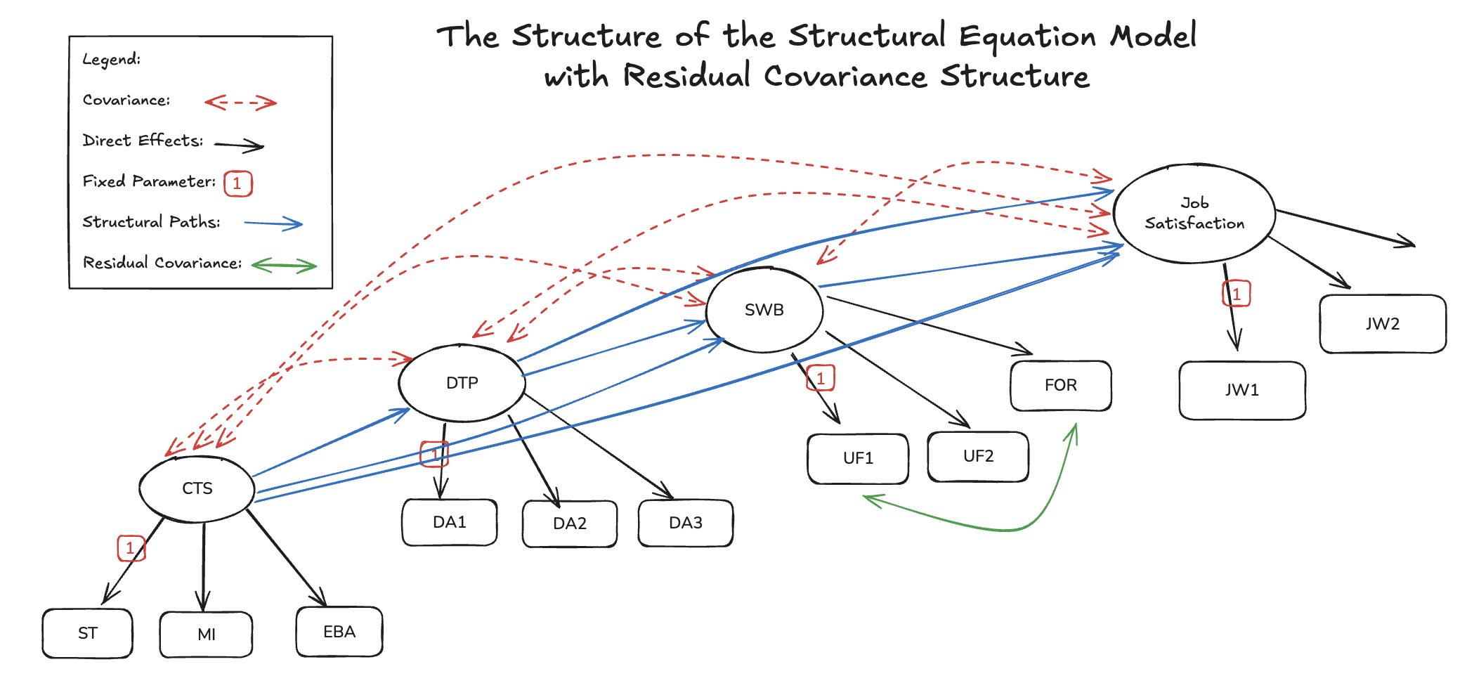
The SEM Regression

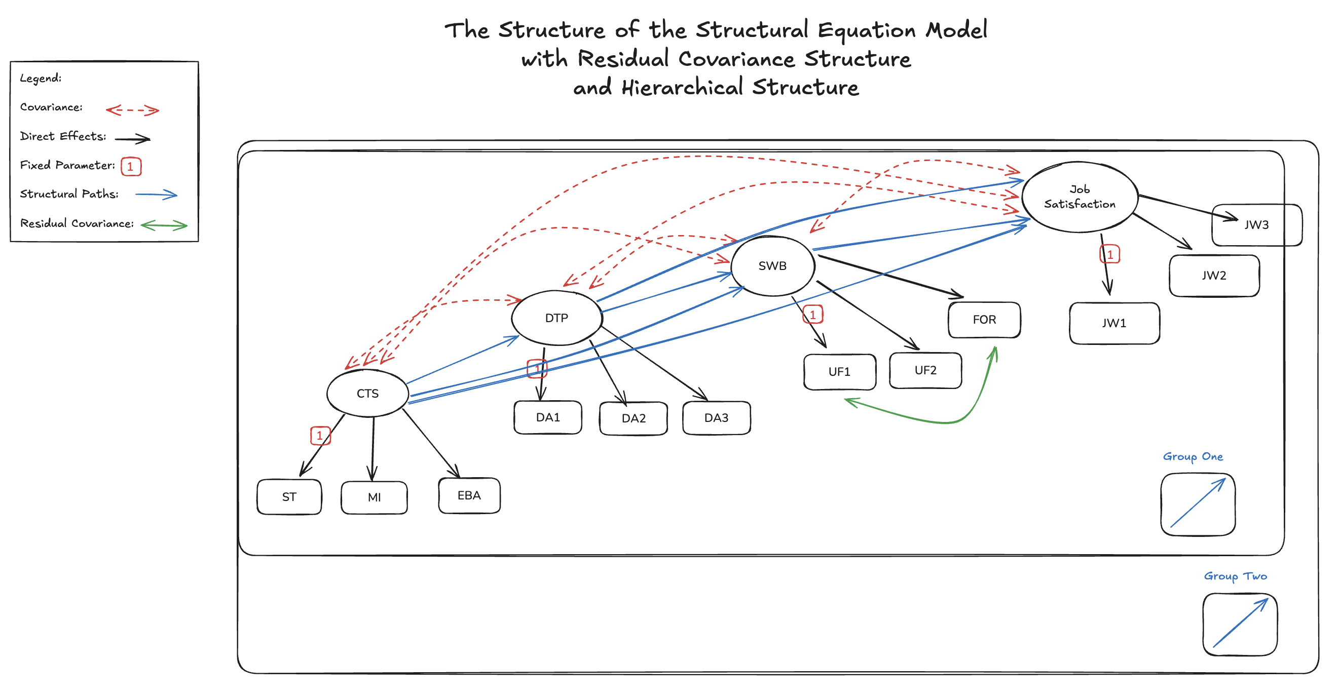
with Residuals Covariance Structures

Bayesian Workflow with SEMs

SEM

with pm.Model(coords=coords) as sem_model_v3:
    
    # --- Factor loadings ---
    lambdas_1 = make_lambda('indicators_1', 'lambdas1', priors=[1, .5])
    lambdas_2 = make_lambda('indicators_2', 'lambdas2', priors=[1, .5])
    lambdas_3 = make_lambda('indicators_3', 'lambdas3', priors=[1, .5])
    lambdas_4 = make_lambda('indicators_4', 'lambdas4', priors=[1, .5])

    Lambda = pt.zeros((12, 4))
    Lambda = pt.set_subtensor(Lambda[0:3, 0], lambdas_1)
    Lambda = pt.set_subtensor(Lambda[3:6, 1], lambdas_2)
    Lambda = pt.set_subtensor(Lambda[6:9, 2], lambdas_3)
    Lambda = pt.set_subtensor(Lambda[9:12, 3], lambdas_4)
    Lambda = pm.Deterministic('Lambda', Lambda)

    latent_dim = len(coords['latent'])

    sd_dist = pm.Exponential.dist(1.0, shape=latent_dim)
    chol, _, _ = pm.LKJCholeskyCov("chol_cov", n=latent_dim, eta=2, sd_dist=sd_dist, compute_corr=True)
    gamma = pm.MvNormal("gamma", 0, chol=chol, dims=("obs", "latent"))

    B = make_B()
    I = pt.eye(latent_dim)
    eta = pm.Deterministic("eta", pt.slinalg.solve(I - B + 1e-8 * I, gamma.T).T)  

    mu = pt.dot(eta, Lambda.T)

    ## Error Terms
    Psi = make_Psi('indicators')
    _ = pm.MvNormal('likelihood', mu=mu, cov=Psi, observed=observed_data)

\[\gamma \sim MvN(0, \Sigma_{\zeta})\] \[\eta = (I-\color{blue}{B})^{-1} \gamma\] \[\mu = \Lambda \eta_i\] \[ \mathbf{y} \mid \eta \sim MvN(\mu, \Psi)\]

Bayesian Workflow with SEMs

SEM Implications

The Beta coefficients encode the directional effects of the latent constructs on one another
High Dysfunction -> Negative Impact on Satisfaction
Factor loadings remain close to 1
Posterior Predictive of the Residuals have Improved

Bayesian Workflow with SEMs

Mean Structures and Marginalising

with pm.Model(coords=coords) as sem_model_mean_structure:
  # --- Factor loadings ---
  lambdas_1 = make_lambda('indicators_1', 'lambdas1', priors=[1, .5])
  lambdas_2 = make_lambda('indicators_2', 'lambdas2', priors=[1, .5])
  lambdas_3 = make_lambda('indicators_3', 'lambdas3', priors=[1, .5])
  lambdas_4 = make_lambda('indicators_4', 'lambdas4', priors=[1, .5])

  Lambda = pt.zeros((12, 4))
  Lambda = pt.set_subtensor(Lambda[0:3, 0], lambdas_1)
  Lambda = pt.set_subtensor(Lambda[3:6, 1], lambdas_2)
  Lambda = pt.set_subtensor(Lambda[6:9, 2], lambdas_3)
  Lambda = pt.set_subtensor(Lambda[9:12, 3], lambdas_4)
  Lambda = pm.Deterministic('Lambda', Lambda)

  sd_dist = pm.Exponential.dist(1.0, shape=4)
  chol, _, _ = pm.LKJCholeskyCov("chol_cov", n=4, eta=2, sd_dist=sd_dist, compute_corr=True)

  Psi_zeta = pm.Deterministic("Psi_zeta", chol.dot(chol.T))
  Psi = make_Psi('indicators')

  B = make_B()
  latent_dim = len(coords['latent'])
  I = pt.eye(latent_dim)
  lhs = I - B + 1e-8 * pt.eye(latent_dim)  # (latent_dim, latent_dim)
  inv_lhs = pm.Deterministic('solve_I-B', pt.slinalg.solve(lhs, pt.eye(latent_dim)), dims=('latent', 'latent1'))

  # Mean Structure
  tau = pm.Normal("tau", mu=0, sigma=0.5, dims="indicators")   # observed intercepts 
  alpha = pm.Normal("alpha", mu=0, sigma=0.5, dims="latent")       # latent means
  mu_y = pm.Deterministic("mu_y", tau + pt.dot(Lambda, pt.dot(inv_lhs, alpha)))

  Sigma_y = pm.Deterministic('Sigma_y', Lambda.dot(inv_lhs).dot(Psi_zeta).dot(inv_lhs.T).dot(Lambda.T) + Psi)
  M = Psi_zeta @ inv_lhs @ Lambda.T @ pm.math.matrix_inverse(Sigma_y)
  eta_hat = pm.Deterministic('eta', alpha + (M @ (observed_data - mu_y).T).T, dims=('obs', 'latent')) 
  _ = pm.MvNormal("likelihood", mu=mu_y, cov=Sigma_y, observed=observed_data)

\[\mu = \tau + \Lambda(1 - B)^{-1}\alpha\] \[\color{blue}{\Sigma_{\mathcal{y}}} = \Psi + \\ \Lambda(I - B)^{-1}\Psi_{\gamma}(I - B)^{T}\Lambda^{T} \]

\[ \mathcal{y} \sim MvN(\mu, \Sigma_{y})\]

Bayesian Workflow with SEMs

Mean Structure Implications

Mean Structure Parameters \(\tau\) show poor identification
Beta coefficients and Factor Loading Estimates consistent with prior models
Posterior Predictive check on Residuals provide evidence of a good fit.

Sensitivity Analysis

Knowing what your Model Implies

Bayesian Workflow with SEMs

Comparing Model Estimates

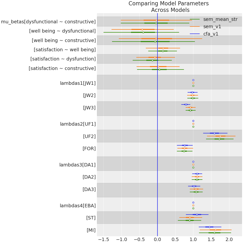
The measurement model is stable: adding the structural paths did not disrupt how the latent variables are measured.
SEM is not introducing distortions into the factor structure.
The hypothesized regression paths are consistent with the observed covariance patterns.
Constructive thought processes: self-talk, visualisation and evaluation of beliefs improve job satisfaction.
Effects are achieved directly and indirectly through overall well being.

Bayesian Workflow with SEMs

Assessing the Indirect Effects

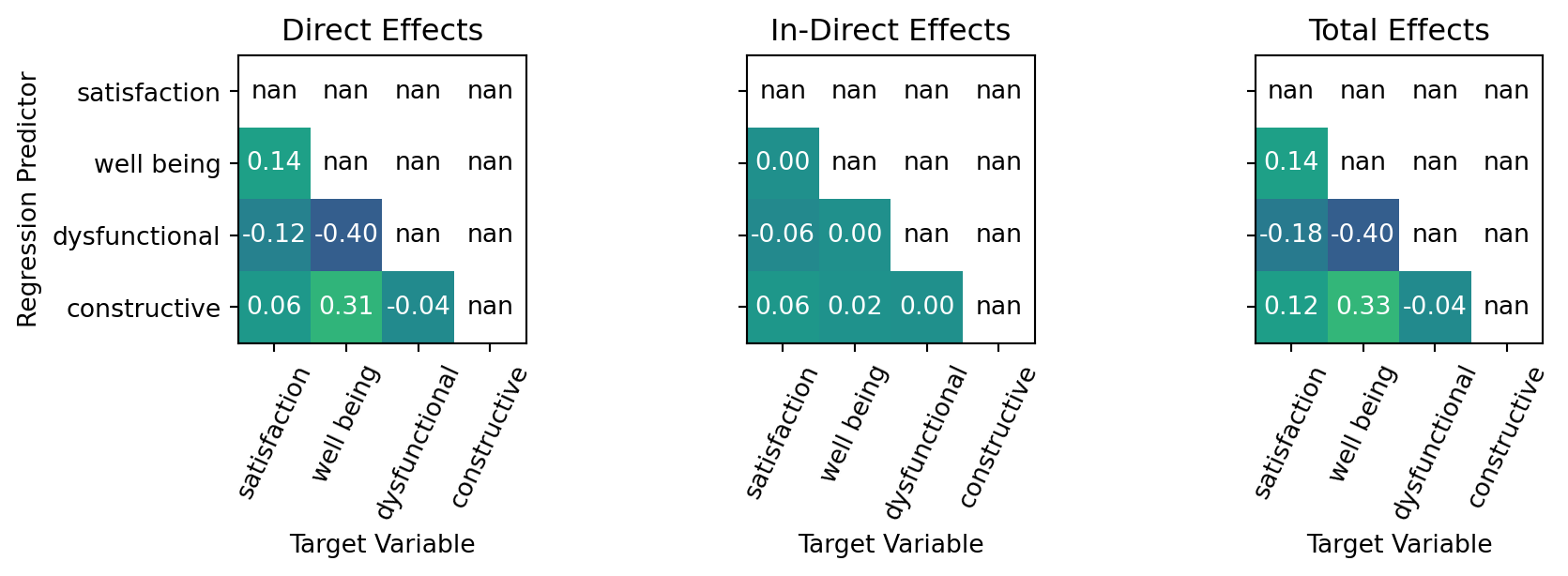
Variations on theme

with Hierarchical Structure

Hierarchies in Code

Complexity and Rich Parameterisation

coords['group'] = ['man', 'woman']
with pm.Model(coords=coords) as sem_model_hierarchical2:
    
    # --- Factor loadings ---
    lambdas_1 = make_lambda('indicators_1', 'lambdas1', priors=[1, .5])
    lambdas_2 = make_lambda('indicators_2', 'lambdas2', priors=[1, .5])
    lambdas_3 = make_lambda('indicators_3', 'lambdas3', priors=[1, .5])
    lambdas_4 = make_lambda('indicators_4', 'lambdas4', priors=[1, .5])

    Lambda = pt.zeros((12, 4))
    Lambda = pt.set_subtensor(Lambda[0:3, 0], lambdas_1)
    Lambda = pt.set_subtensor(Lambda[3:6, 1], lambdas_2)
    Lambda = pt.set_subtensor(Lambda[6:9, 2], lambdas_3)
    Lambda = pt.set_subtensor(Lambda[9:12, 3], lambdas_4)
    Lambda = pm.Deterministic('Lambda', Lambda)

    sd_dist = pm.Exponential.dist(1.0, shape=4)
    chol, _, _ = pm.LKJCholeskyCov("chol_cov", n=4, eta=2, sd_dist=sd_dist, compute_corr=True)

    Psi_zeta = pm.Deterministic("Psi_zeta", chol.dot(chol.T))
    Psi = make_Psi('indicators')

    Bs = []
    for g in coords["group"]:
        B_g = make_B(group_suffix=f"_{g}")  # give group-specific names
        Bs.append(B_g)
    B_ = pt.stack(Bs)

    latent_dim = len(coords['latent'])
    I = pt.eye(latent_dim)

    # invert (I - B_g) for each group
    inv_I_minus_B = pt.stack([
        pt.slinalg.solve(I - B_[g] + 1e-8 * I, I)
        for g in range(len(coords["group"]))
    ])

    # Mean Structure
    tau = pm.Normal("tau", mu=0, sigma=0.5, dims=('group', 'indicators'))   # observed intercepts 
    alpha = pm.Normal("alpha", mu=0, sigma=0.5, dims=('group', 'latent'))       # latent means
    M = pt.matmul(Lambda, inv_I_minus_B)  # group, indicators latent
    mu_latent = pt.matmul(alpha[:, None, :], M.transpose(0, 2, 1))[:,:,0] # shape handling dummy axis and transpose M -> group, latent, indicators
    mu_y = pm.Deterministic("mu_y", tau + mu_latent) # size = group, indicators

    Sigma_y = []
    for g in range(len(coords['group'])):
        inv_lhs = inv_I_minus_B[g]
        Sigma_y_g = Lambda @ inv_lhs @ Psi_zeta @ inv_lhs.T @ Lambda.T + Psi
        Sigma_y.append(Sigma_y_g)
    Sigma_y = pt.stack(Sigma_y)
    _ = pm.MvNormal("likelihood", mu=mu_y[grp_idx], cov=Sigma_y[grp_idx])

\[ \mu_g = \tau_{g} + \Lambda(1 - B_{g})^{-1}\alpha_{g}\] \[\Sigma_{\mathcal{y}} = \Psi + \\ \Lambda(I - \color{blue}{B_{g}})^{-1}\Psi_{\gamma}(I - \color{blue}{B_{g}})^{T}\Lambda^{T} \]

\[ \mathcal{y} \sim MvN(\mu_{g}, \Sigma_{y}^{g})\]

Validating Model Implications

The Do-Operator and Parameter Recovery


# Generating data from model by fixing parameters
fixed_parameters = {
 "mu_betas_man": [0.1, 0.5, 2.3, 0.9, 0.6, 0.8],
 "mu_betas_woman": [0.3, 0.2, 0.7, 0.8, 0.6, 1.2], 
 "tau": [[-0.822,  1.917, -0.743, -0.585, -1.095,  2.207, -0.898, -0.99 ,
        1.872, -0.044, -0.035, -0.085], [-0.882,  1.816, -0.828, -1.319,
        0.202,  1.267, -1.784, -2.112,  3.705, -0.769,  2.048, -1.064]],
 "lambdas1_": [1, .8, .9],
 "lambdas2_": [1, .9, 1.2],
 "lambdas3_": [1, .95, .8],
 "lambdas4_": [1, 1.4, 1.1],
 "alpha": [[ 0.869,  0.242,  0.314, -0.175], [0.962,  1.036,  0.436,  0.166]], 
 "chol_cov": [0.696, -0.096,  0.23 , -0.3  , -0.385,  0.398, -0.004,  0.043,
       -0.037,  0.422], 
"Psi_cov_": [0.559, 0.603, 0.666, 0.483, 0.53 , 0.402, 0.35 , 0.28 , 0.498,
       0.494, 0.976, 0.742], 
"Psi_cov_beta": [0.029]
}
with pm.do(sem_model_hierarchical2, fixed_parameters) as synthetic_model:
   idata = pm.sample_prior_predictive(random_seed=1000) # Sample from prior predictive distribution.
   synthetic_y = idata['prior']['likelihood'].sel(draw=0, chain=0)

# Infer parameters conditioned on observed data
with pm.observe(sem_model_hierarchical2, {"likelihood": synthetic_y}) as inference_model:
   idata = pm.sample(random_seed=100, nuts_sampler='numpyro', chains=4, draws=500)

Parameter Recovery

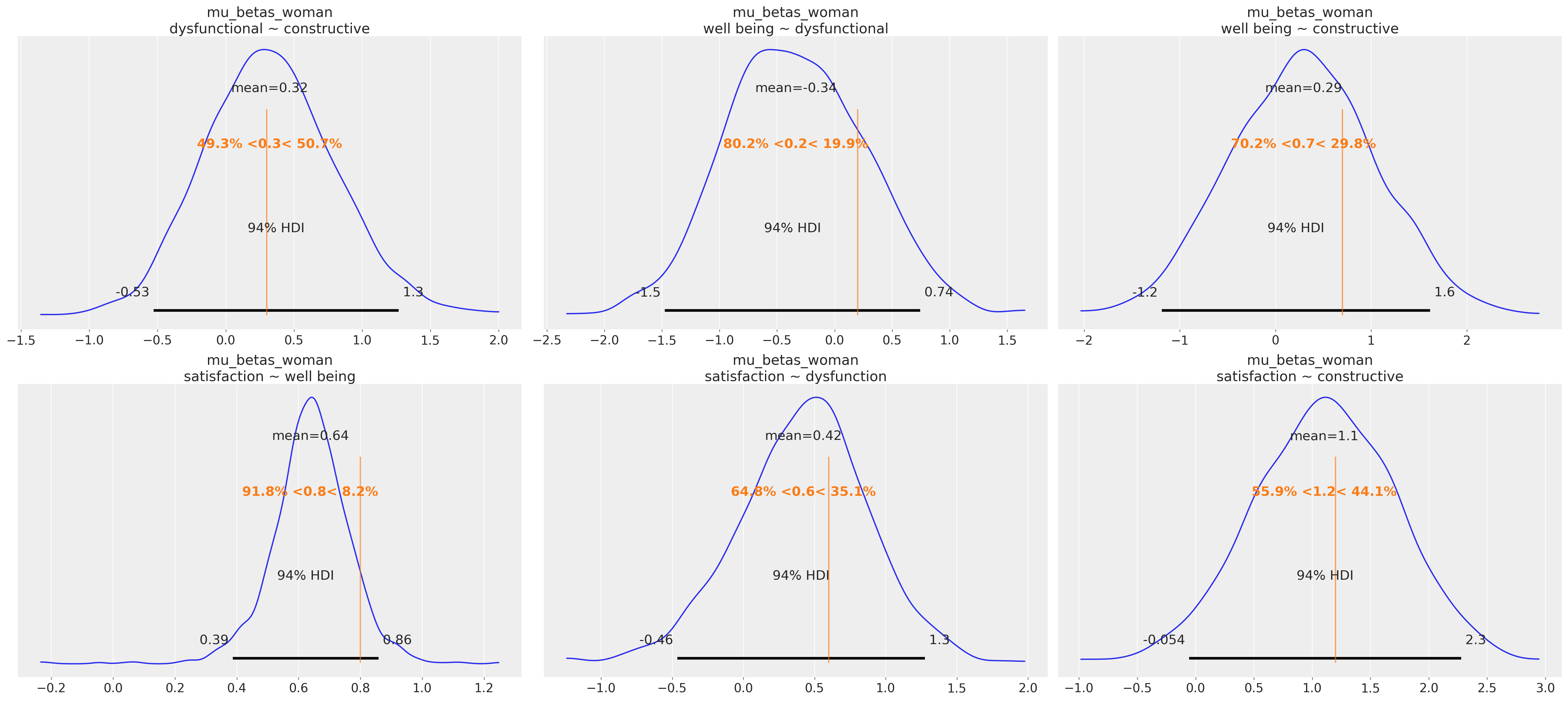
Complex models require proper validation methods. Parameter recovery methods are the best way to test the model’s ability to identify the correct effects.

Workflow and Craft

Craft as Discovery

“Abandon the idea of predetermination, the shaping force of your intentions…rely less on the priority of your intentions and more on the immediacy of writing… You’ll see that some of your sentences are still conjectural… start noticing the thoughts and implications surrounding them.” - Verlyn Klinkenborg in Several Short Sentences about Writing”

Modeling, like writing, is an act of exploration.

Expect surprises and anomalies—they teach more than preconceptions.

Embrace uncertainty; allow the data to guide the process.

Craft as Discipline

” [T]he goal is to represent the systematic relationships between the variables and between the variables and the parameters … Discrepancies between the model and data can be used to learn about the ways in which the model is inadequate for the scientific purposes at hand, and thus to motivate expansions and changes to the model … a model is a story of how the data could have been generated; the fitted model should therefore be able to generate synthetic data that look like the real data; failures to do so in important ways indicate faults in the model.” - Gelman & Shalizi in Philosophy and the practice of Bayesian statistics

Building statistical models is inherently iterative and expansionary

Assumptions are encoded transparently and their implications are assessed for cogency

Where our assumptions fail, they are revised or rejected. Building confidence and clarity.

The process yields compelling, justifiable conclusions worthy of your work.

Conclusion: Workflow as Craft

“Here, in short, is what i want to tell you. Know what each sentence says, What it doesn’t say, And what it implies. Of these, the hardest is know what each sentence actually says” - V. Klinkenborg

In modelling, as in writing, clarity emerges through revision.

The Bayesian workflow with PyMC teaches us to listen to our models — to read them aloud through simulation, recovery, and critique.

Each iteration reveals what the model truly says, what it hides, and what it implies.

Craft lies in that attention — in resisting flattening automation, and choosing understanding over throughput.

Through this care, our models become not only more compelling, but more robust — resilient to noise, misfit, and misuse.