Multilevel Regression and Post-Stratification
Stratum Specific effect modification with Bambi
2025-05-14
Preliminaries
Intro
- I’m a data scientist at Personio
- Bayesian statistician,
- Reformed philosopher and logician.
- Website: https://nathanielf.github.io/
Disclaimer
None of Personio’s data was used in this presentation

QR Website Code
Code or it didn’t Happen
The worked examples used here can be found here
Regression: What are we even doing?
\[\hat{y_{i}} = \alpha + \beta_{1}X_{1} ... \beta_{n}X_{n}\]
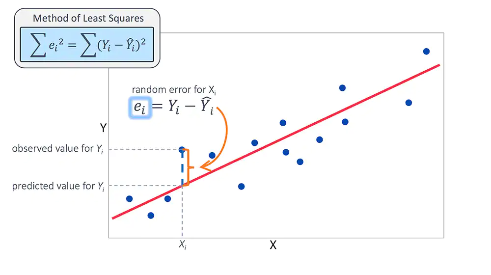
Assume \(y = \hat{y_{i}} + \epsilon\) where \(E(\epsilon) = 0\)
\[ E[y | X = x] = \alpha + \beta_{1}X_{1} ... \beta_{n}X_{n}\]
\[ y \sim Normal(\hat{y_{i}}, \sigma) \]
Regression: What are we even doing?
m0 = smf.ols('np.log(hwage) ~ job +  educ', data=df).fit()
m1 = smf.ols('np.log(hwage) ~ job + educ + male ', data=df).fit()
pred = m0.predict(['software_engineer', 'college'])
pred1 = m1.predict(['software_engineer', 'college', 1])
diff = predc - pred1
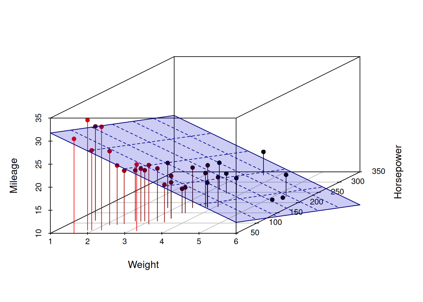
As we add more covariates we add more combinatorial branches which define the available strata across our population of interest.
A fitted regression model allows us to explore the conditional branching probabilities.

Regression as Weighting Adjustment
Regression automates the more manual re-weighting
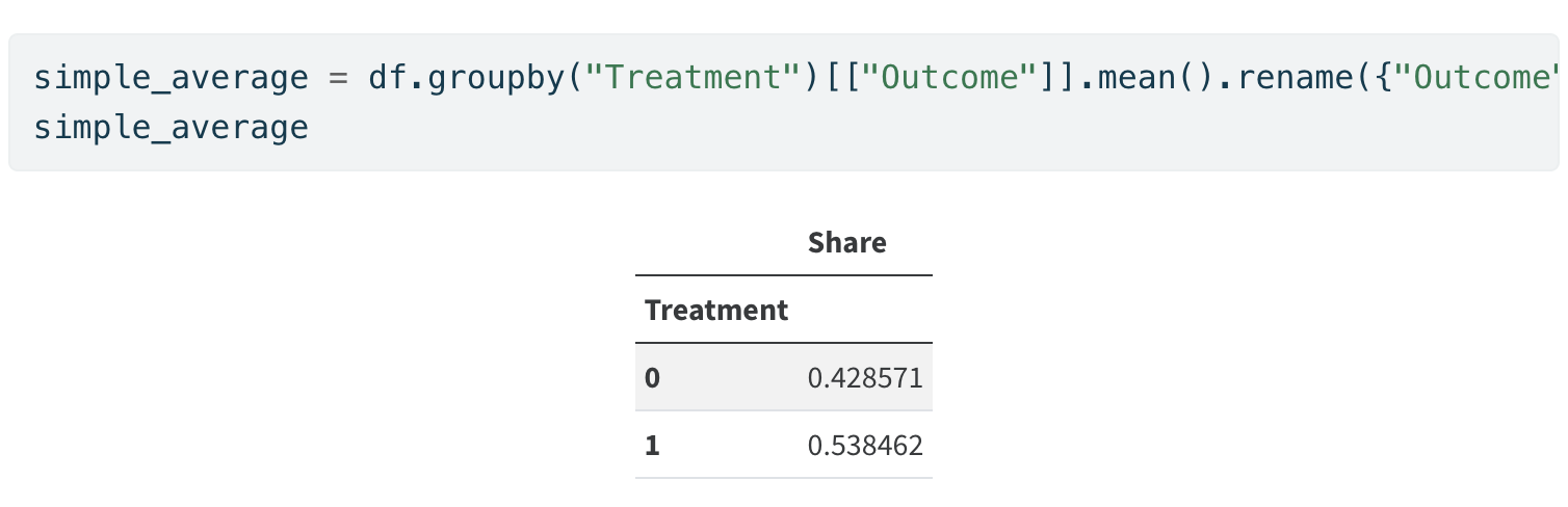
Simple Unweighted Average
Regression as Weighting Adjustment
Regression automates the more manual re-weighting
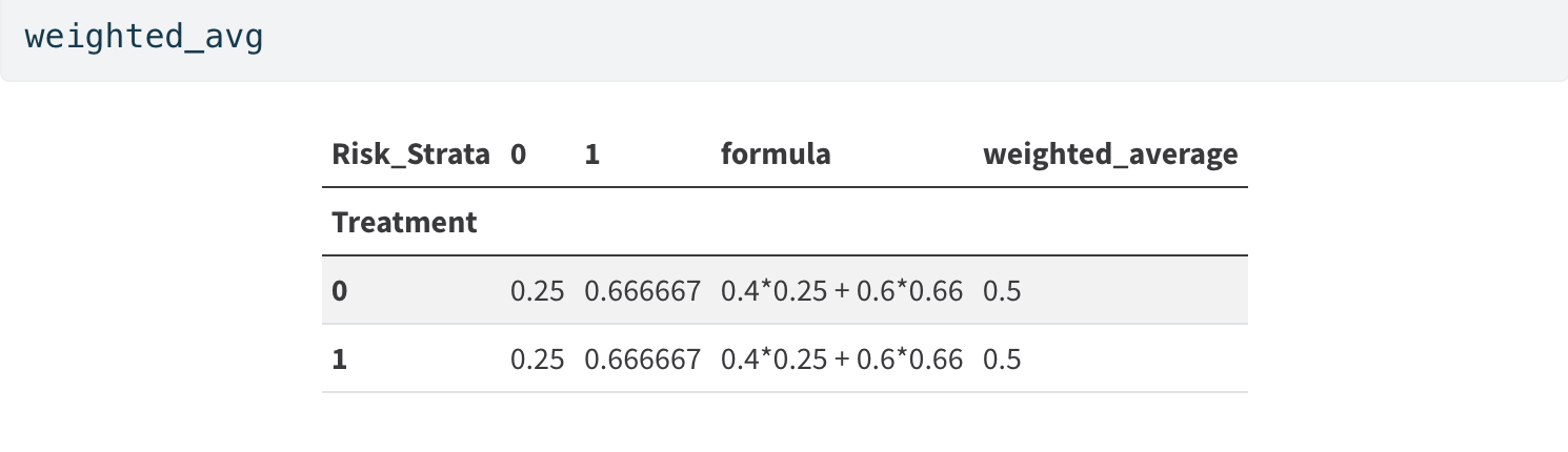
Weighted Average
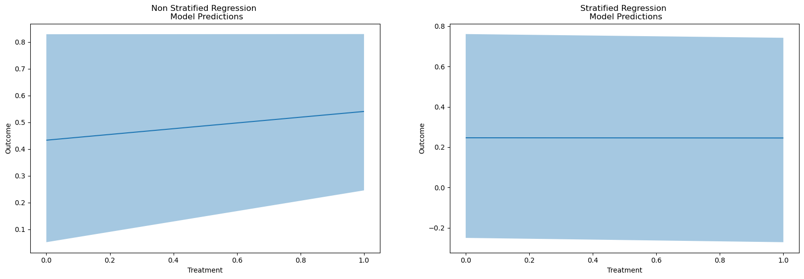
Regression as Effect Modification
reg = bmb.Model("Outcome ~ 1 + Treatment", df)
results = reg.fit()

reg_strata = bmb.Model("""Outcome ~ 1 + Treatment + Risk_Strata
+ Treatment_x_Risk_Strata""", df)
results_strata = reg_strata.fit()
bmb.interpret.plot_predictions(reg, results, conditional=["Treatment"])
bmb.interpret.plot_predictions(reg_strata, results_strata, conditional=["Treatment"])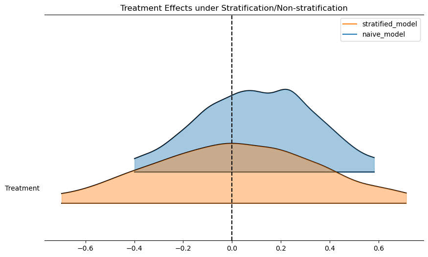
The Data
We examine a comprehensive YouGov poll on whether employers should cover abortion in their coverage plans.
We select a biased subsample.
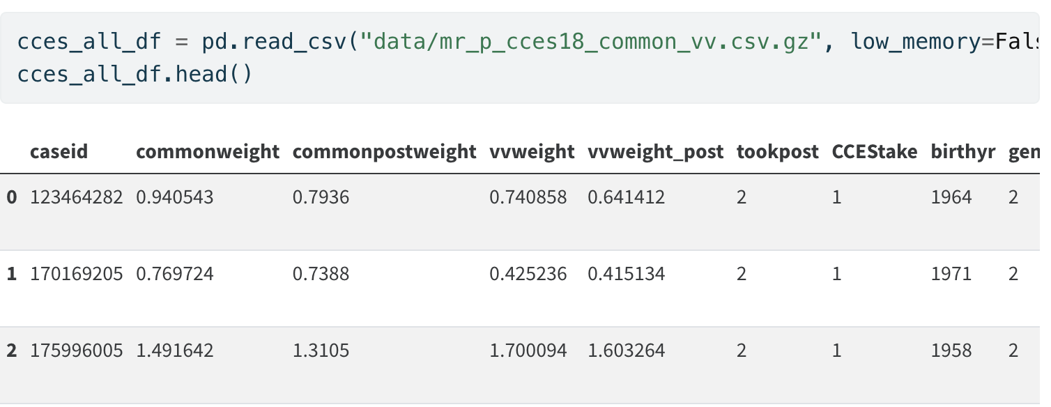
State Level Data
Deliberate Bias
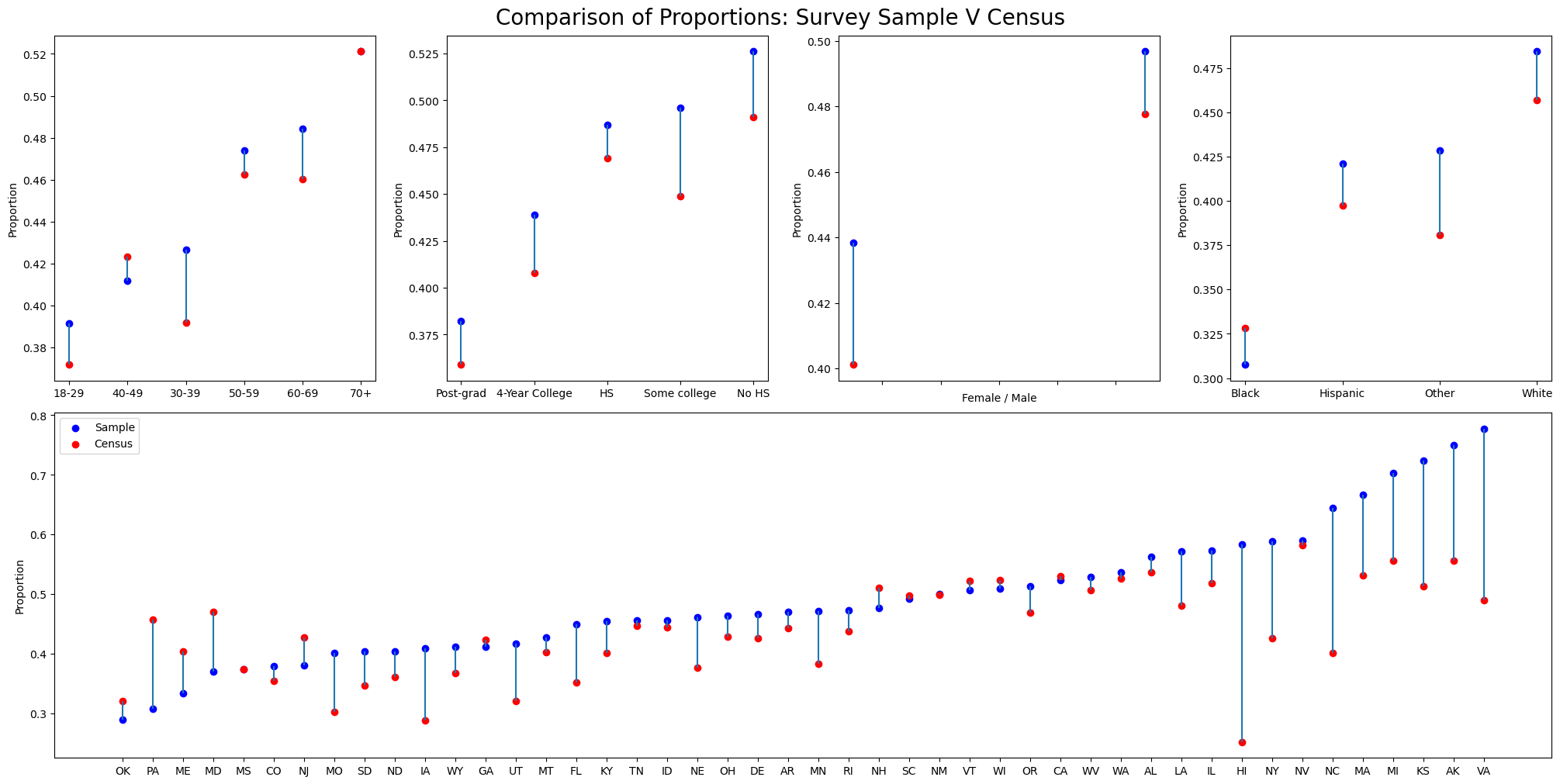
Illustrated differences in vote share by demographics
Prep Data for Modelling
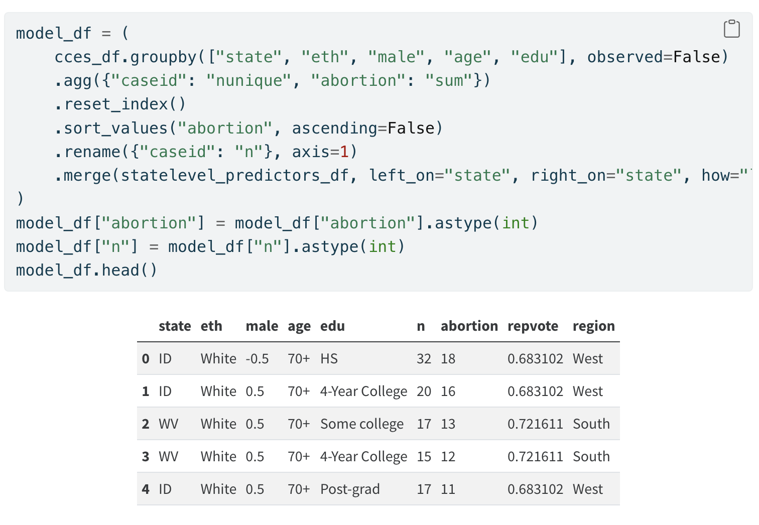
Aggregate Across Strata
Plotting Implications
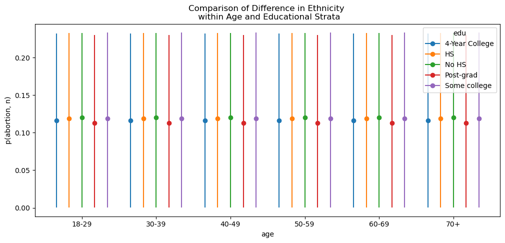
Exploratory Interaction Effects
Plotting Implications
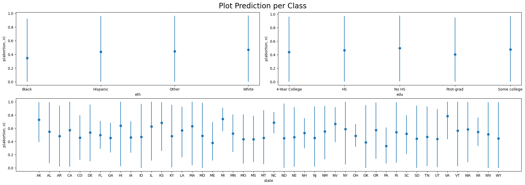
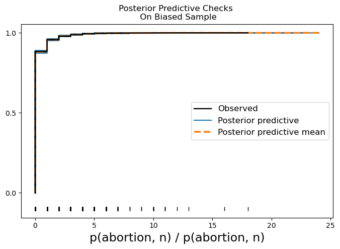
Posterior Predictive By Class
Investigating Marginal Contrasts
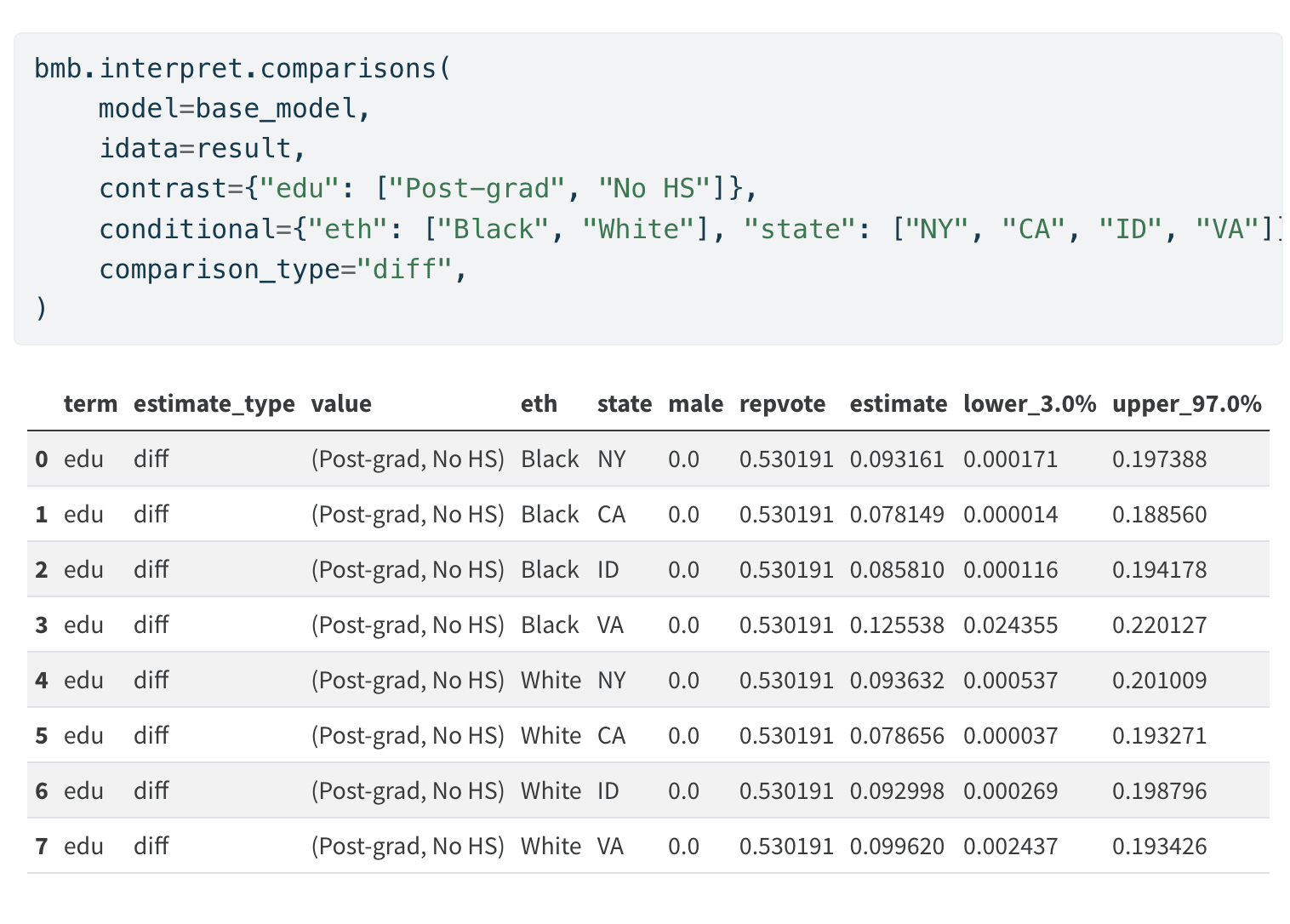
Marginal Differences
The Model in Code
Fitting the model to the biased sample:
formula = """ p(abortion, n) ~ (1 | state) + (1 | eth) + (1 | edu)
 + male + repvote  + (1 | male:eth) + (1 | edu:age) + (1 | edu:eth)"""

model_hierarchical = bmb.Model(formula, model_df, family="binomial")
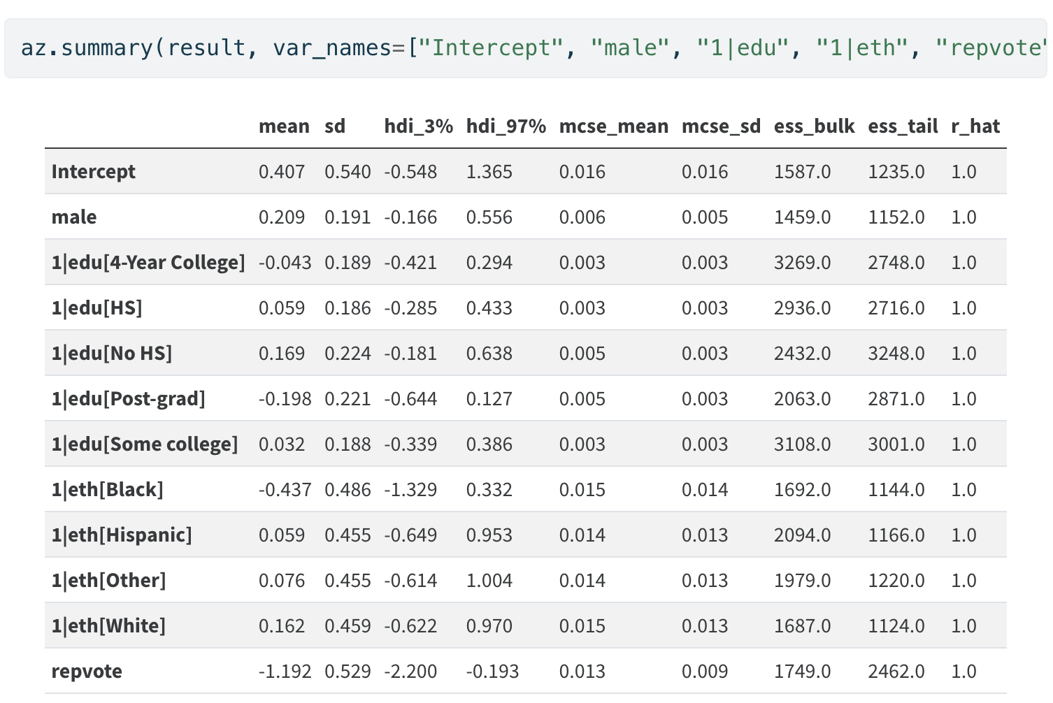
Learning the Bias
The Model Derived Coefficients
Predicting Vote Share
Using the Biased Model
new_data = (new_data.merge(
    new_data.groupby("state").agg({"n": "sum"})
    .reset_index()
    .rename({"n": "state_total"}, axis=1)
)
)
new_data["state_percent"] = new_data["n"] / new_data["state_total"]
new_data.head()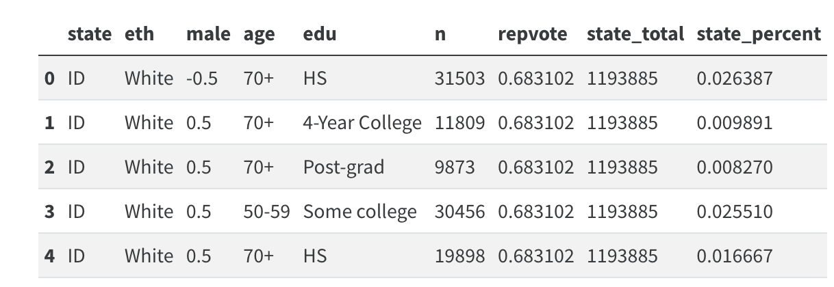
Population by Strata
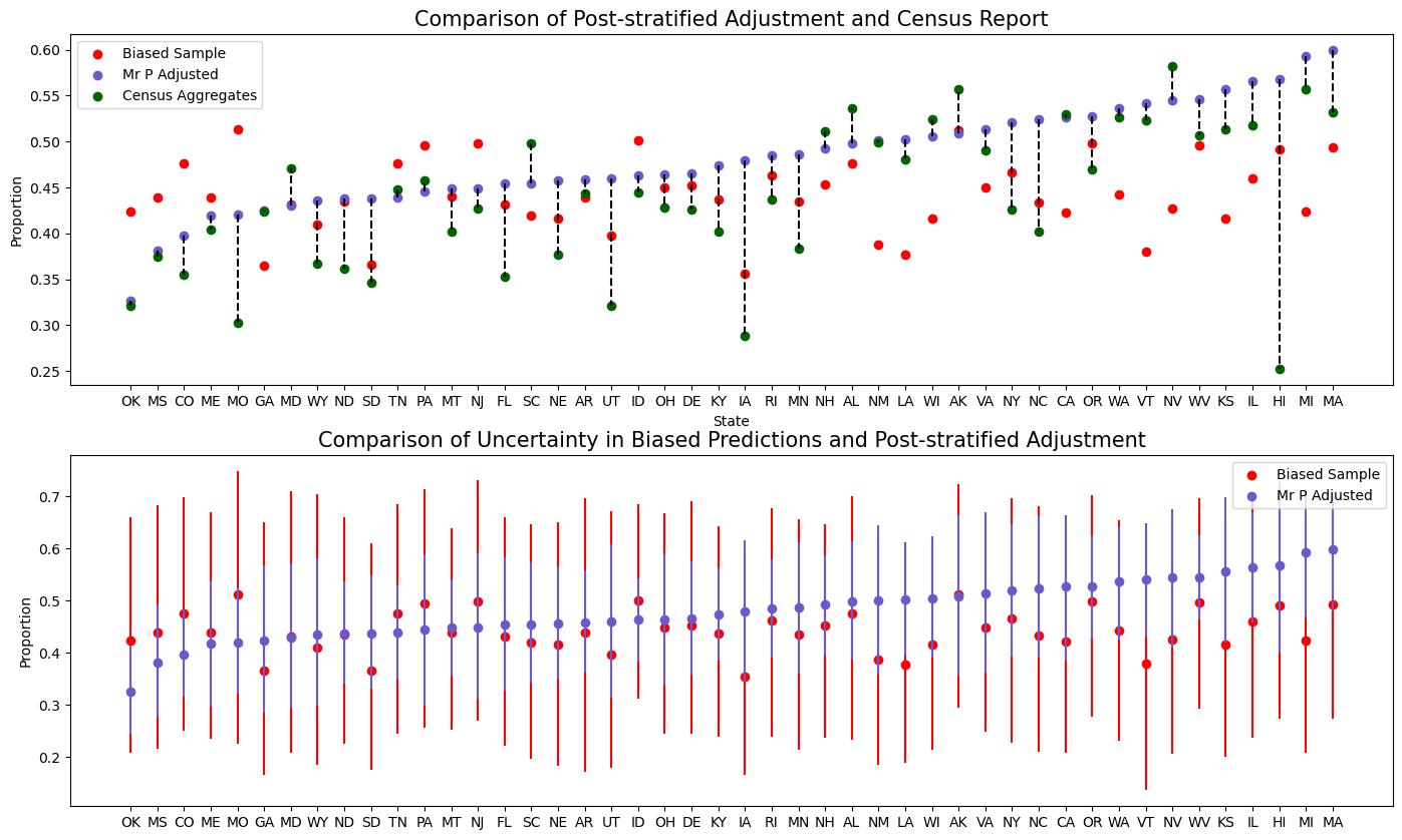
Comparing Adjusted and Raw Predictions
Derived state level predictions using the biased sample and the corrected values.
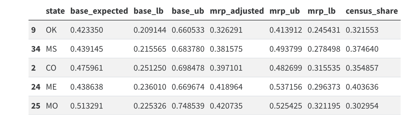
Adjusted Predictions
Comparing Adjusted and Raw Predictions
Comparing Predictions to Adjusted Predictions