Model Evaluation and Discrete Choice Scenarios

Bayesian Mixer London

Nathaniel Forde

Data Science @ Personio

and Open Source Contributor @ PyMC

3/26/24

Preliminaries

I am not an Economist

• I’m a data scientist at Personio - where we work on cool problems ranging across themes of:
  • revenue optimisation
  • customer churn
  • experimentation
  • survey design
  • product analytics
• Bayesian statistician, reformed philosopher and logician.
• Website: https://nathanielf.github.io/

Disclaimer

None of Personio’s data was used in this presentation

Code or it didn’t Happen

The worked examples used here can be found here

The Pitch

Merely Predictive Models are inadequate decision making tools in product demand analysis.

Accept no substitutes for bayesian discrete choice models and causal inference.

Agenda

• History and Conceptual Background

• A Naive Utilty Model

• An Augmented Model

• Adding Correlation Structure

• Counterfactual Questions

• Individual Heterogenous Utility

• Conclusion
  • The World in the Model

History and Background

A brief survey of historical use-cases and the kinds of problems Bayesian discrete choice models can solve.

McFadden and BART

“Transport projects involve sinking money in expensive capital investments, which have a long life and wide repercussions. There is no escape from the attempt both to estimate the demand for their services over twenty or thirty years and to assess their repercussions on the economy as a whole.” - Denys Munby, Transport, 1968 ”

Bay Area Rapid Transit

Dublin Metrolink

Revealed Preference and Predicting Demand

Self Centred Utility Maximisers?

• The assumption of revealed preference theory is that if a person chooses A over B then their latent subjective utility for A is greater than for B.

• Survey data estimated about 15% of users would adopt the newly introduced BART system. McFadden’s random utility model estimated 6%.

• He was right.

• Copernican Shift: He estimated utility to predict choice, rather than infer utility from stated choice.

General Applicability of Choice Problems

• These models offer the possibility of predicting choice in diverse domains: policy, brand, school, car and partners.

• Question: What are the attributes that drive these choices? How well are they measurable?

• Question: How do changes in these attributes influence the predicted market demand for these choices?

Note on Model Evaluation

Replicating the Super Soldier Program

Note on Model Evaluation

Replicating the Super Soldier Program

Bayesian Models aim to replicate the DGP holistically

A Naive Model

A baseline model for incorporating item specific utilities to predict market share.

Choice: The Data

Gas Central Heating and Electrical Central Heating described by their cost of installation and operation.

choice_id	chosen	ic_gc	oc_gc	…	oc_ec
1	gc	866	200	…	542
2	ec	802	195	…	510
3	er	759	203	…	495
4	gr	789	220	…	502

Choice: A Naive Model

Underspecified Utilities

Let there be five goods described by their cost of installation and operation.

\[ \begin{split} \overbrace{\begin{pmatrix} \color{green}{u_{gc}} \\ \color{green}{u_{gr}} \\ \color{green}{u_{ec}} \\ \color{green}{u_{er}} \\ \color{green}{u_{hp}} \\ \end{pmatrix}}^{utility} = \begin{pmatrix} gc_{ic} & gc_{oc} \\ gr_{ic} & gr_{oc} \\ ec_{ic} & ec_{oc} \\ er_{ic} & er_{oc} \\ hp_{ic} & hp_{oc} \\ \end{pmatrix} \overbrace{\begin{pmatrix} \color{blue}{\beta_{ic}} \\ \color{blue}{\beta_{oc}} \\ \end{pmatrix}}^{parameters} \end{split} \]

Choice: A Naive Model

The utility calculation is fundamentally comparative. \[ \begin{split} \begin{pmatrix} \color{green}{u_{gc}} \\ \color{green}{u_{gr}} \\ \color{green}{u_{ec}} \\ \color{green}{u_{er}} \\ \color{red}{\overbrace{0}^{\text{outside good}}} \\ \end{pmatrix} = \begin{pmatrix} gc_{ic} & gc_{oc} \\ gr_{ic} & gr_{oc} \\ ec_{ic} & ec_{oc} \\ er_{ic} & er_{oc} \\ \color{red}{0} & \color{red}{0} \\ \end{pmatrix} \begin{pmatrix} \color{blue}{\beta_{ic}} \\ \color{blue}{\beta_{oc}} \\ \end{pmatrix} \end{split} \]

We zero out one category in the data set to represent the “outside good” for comparison. Similar to dummy variables in Regression, this is required for the model to be identified.

Choice: A Naive Model

Utility determines choice probability of choice:

\[\text{softmax}(\color{green}{u})_{j} = \frac{\exp(\color{green}{u_{j}})}{\sum_{q=1}^{J}\exp(\color{green}{u_{q}})}\]

choices determine market share where:

\[ s_{j}(\mathbf{\color{blue}{\beta}}) = P(\color{green}{u_{j}} > \color{green}{u_{k}}; ∀k ̸= j) \]

Choice: Estimation

The model is traditionally estimated with maximum likelihood caclulations.

\[ L(\color{blue}{\beta}) = \prod s_{j}(\mathbf{\color{blue}{\beta}}) \]

or taking the log:

\[ l(\color{blue}{\beta}) = \sum log(s_{j}(\mathbf{\color{blue}{\beta}})) \] \[ \text{ We find: } \underset{\color{blue}{\beta}}{\mathrm{argmax}} \text{ } l(\color{blue}{\beta}) \]

Results are often brittle!

Choice: Bayesian Estimation

To evaluate the integrals in the Bayesian model we use MCMC to estimate conditional probabilities of the joint distribution.

\[\underbrace{\color{blue}{\beta}}_{\text{prior draws}} \sim Normal(0, 1) \]

\[ \underbrace{p(\color{blue}{\beta} | D)}_{\text{posterior draws}} = \frac{p(\mathbb{\color{blue}{\beta}})p(D | \color{blue}{\beta} )}{\int_{i}^{n} p(D | \mathbf{\color{blue}{\beta_{i}}})p(\mathbf{\color{blue}{\beta_{i}}}) } \]

Priors can be used flexibly regularise and improve reliability of estimation across structural causal models.

The Naive Model in Code

with pm.Model(coords=coords) as model_1:
    ## Priors for the Beta Coefficients
    beta_ic = pm.Normal("beta_ic", 0, 1)
    beta_oc = pm.Normal("beta_oc", 0, 1)

    ## Construct Utility matrix and Pivot
    u0 = beta_ic * wide_heating_df["ic.ec"] + beta_oc * wide_heating_df["oc.ec"]
    u1 = beta_ic * wide_heating_df["ic.er"] + beta_oc * wide_heating_df["oc.er"]
    u2 = beta_ic * wide_heating_df["ic.gc"] + beta_oc * wide_heating_df["oc.gc"]
    u3 = beta_ic * wide_heating_df["ic.gr"] + beta_oc * wide_heating_df["oc.gr"]
    u4 = np.zeros(N)  # Outside Good
    s = pm.math.stack([u0, u1, u2, u3, u4]).T

    ## Apply Softmax Transform
    p_ = pm.Deterministic("p", pm.math.softmax(s, axis=1), dims=("obs", "alts_probs"))

    ## Likelihood
    choice_obs = pm.Categorical("y_cat", p=p_, observed=observed, dims="obs")

Interpreting the Model Coefficients

Rate of Substitution

The beta coefficients in the model are interpreted as weights of utility. However, the precision in these latent terms is relative to the variance of unobserved factors.

The utility scale is not fixed, but the ratio \(\frac{\beta_{ic}}{\beta_{oc}}\) is invariant.

Rate of Substitution

Model Posterior Predictive Fits

The model fit fails to recapture the observed data points

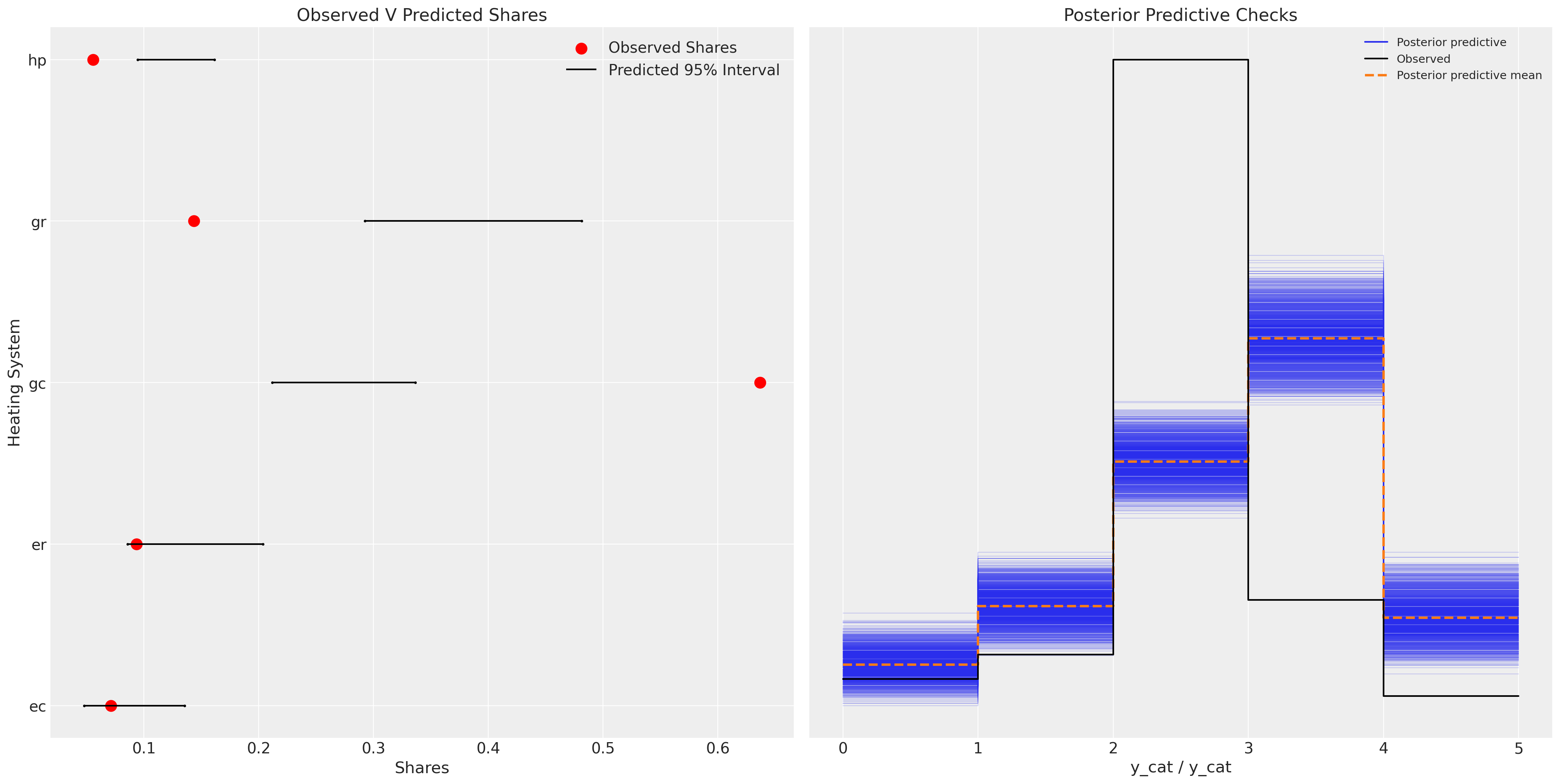
Model Fit

Augmenting the Model

Model now incorporates specification of the mean utilities per item.

Augmenting the Model:

Product Specific Intercepts

\[ \begin{split} \begin{pmatrix} \color{red}{u_{gc}} \\ \color{purple}{u_{gr}} \\ \color{orange}{u_{ec}} \\ \color{teal}{u_{er}} \\ 0 \end{pmatrix} = \begin{pmatrix} \color{red}{\alpha_{gc}} + \color{blue}{\beta_{ic}}gc_{ic} + \color{blue}{\beta_{oc}}gc_{oc} \\ \color{purple}{\alpha_{gr}} + \color{blue}{\beta_{ic}}gr_{ic} + \color{blue}{\beta_{oc}}gr_{oc} \\ \color{orange}{\alpha_{ec}} + \color{blue}{\beta_{ic}}ec_{ic} + \color{blue}{\beta_{oc}}ec_{oc} \\ \color{teal}{\alpha_{er}} + \color{blue}{\beta_{ic}}er_{ic} + \color{blue}{\beta_{oc}}er_{oc} \\ 0 + 0 + 0 \end{pmatrix} \end{split} \]

Augmenting the Model:

with pm.Model(coords=coords) as model_2:
    ## Priors for the Beta Coefficients
    beta_ic = pm.Normal("beta_ic", 0, 1)
    beta_oc = pm.Normal("beta_oc", 0, 1)
    alphas = pm.Normal("alpha", 0, 1, dims="alts_intercepts")

    ## Construct Utility matrix and Pivot using an intercept per alternative
    u0 = alphas[0] + beta_ic * wide_heating_df["ic.ec"] + beta_oc * wide_heating_df["oc.ec"]
    u1 = alphas[1] + beta_ic * wide_heating_df["ic.er"] + beta_oc * wide_heating_df["oc.er"]
    u2 = alphas[2] + beta_ic * wide_heating_df["ic.gc"] + beta_oc * wide_heating_df["oc.gc"]
    u3 = alphas[3] + beta_ic * wide_heating_df["ic.gr"] + beta_oc * wide_heating_df["oc.gr"]
    u4 = np.zeros(N)  # Outside Good
    s = pm.math.stack([u0, u1, u2, u3, u4]).T

    ## Apply Softmax Transform
    p_ = pm.Deterministic("p", pm.math.softmax(s, axis=1), dims=("obs", "alts_probs"))

    ## Likelihood
    choice_obs = pm.Categorical("y_cat", p=p_, observed=observed, dims="obs")

Augmenting the Model:

Model Structure

Augmenting the Model

Posterior Predictions

Model Fit

Independence of Irrelevant Alternatives

New Products Cannibalise Equally from all Alternatives

• Suppose a market choice between transport modes is determined by the above model.
• Red Bus or Car are you initial Options. Assume \(s_{\color{red}{bus}}(\beta) = s_{car}(\beta)\). Market Share is 50% to each option.
• Introduce the Blue Bus Option, then the Independent characteristics of the utility specification implies that \(s_{\color{red}{bus}}(\beta) = s_{car}(\beta) = s_{\color{blue}{bus}}(\beta)\)
• This implies an implausible substitution pattern for real markets.¹

1. What kind of Monster have we Created!?

Adding Correlation Structure

Model tries to account for pathological patterns of sustitution between goods by incorporating covariance structures.

Adding Correlation Structure

Dependence in Market Share

\[ \alpha_{i} \sim Normal(\mathbf{0}, \color{brown}{\Gamma}) \]

\[ \begin{split} \begin{pmatrix} \color{red}{u_{gc}} \\ \color{purple}{u_{gr}} \\ \color{orange}{u_{ec}} \\ \color{teal}{u_{er}} \\ 0 \end{pmatrix} = \begin{pmatrix} \color{red}{\alpha_{gc}} + \color{blue}{\beta_{ic}}gc_{ic} + \color{blue}{\beta_{oc}}gc_{oc} \\ \color{purple}{\alpha_{gr}} + \color{blue}{\beta_{ic}}gr_{ic} + \color{blue}{\beta_{oc}}gr_{oc} \\ \color{orange}{\alpha_{ec}} + \color{blue}{\beta_{ic}}ec_{ic} + \color{blue}{\beta_{oc}}ec_{oc} \\ \color{teal}{\alpha_{er}} + \color{blue}{\beta_{ic}}er_{ic} + \color{blue}{\beta_{oc}}er_{oc} \\ 0 + 0 + 0 \end{pmatrix} \end{split} \]

Adding Correlation Structure

Priors on Parameters determine Market Structure

\[ \begin{split} \color{brown}{\Gamma} = \begin{pmatrix} \color{red}{1} , \gamma , \gamma , \gamma \\ \gamma , \color{blue}{1} , \gamma , \gamma \\ \gamma , \gamma , \color{orange}{1} , \gamma \\ \gamma , \gamma , \gamma , \color{teal}{1} \end{pmatrix} \end{split} \]

Adding Correlation Structure

with pm.Model(coords=coords) as model_3:
    beta_ic = pm.Normal("beta_ic", 0, 1)
    beta_oc = pm.Normal("beta_oc", 0, 1)

    beta_income = pm.Normal("beta_income", 0, 1 dims="alts_intercepts")

    chol, corr, stds = pm.LKJCholeskyCov(
        "chol", n=4, eta=2.0, 
        sd_dist=pm.Exponential.dist(1.0, shape=4)
    )
    alphas = pm.MvNormal("alpha", mu=0, chol=chol, dims="alts_intercepts")

    u0 = (
        alphas[0]
        + beta_ic * wide_heating_df["ic.gc"]
        + beta_oc * wide_heating_df["oc.gc"]
        + beta_income[0] * wide_heating_df["income"]
    )
    u1 = (
        alphas[1]
        + beta_ic * wide_heating_df["ic.gc"]
        + beta_oc * wide_heating_df["oc.gc"]
        + beta_income[1] * wide_heating_df["income"]
    )
    u2 = (
        alphas[2]
        + beta_ic * wide_heating_df["ic.gc"]
        + beta_oc * wide_heating_df["oc.gc"]
        + beta_income[2] * wide_heating_df["income"]
    )
    u3 = (
        alphas[3]
        + beta_ic * wide_heating_df["ic.gr"]
        + beta_oc * wide_heating_df["oc.gr"]
        + beta_income[3] * wide_heating_df["income"]
    )
    u4 = np.zeros(N)  # pivot
    s = pm.math.stack([u0, u1, u2, u3, u4]).T

    p_ = pm.Deterministic("p", pm.math.softmax(s, axis=1), dims=("obs", "alts_probs"))
    choice_obs = pm.Categorical("y_cat", p=p_, observed=observed, dims="obs")

Adding Correlation Structure

Correlation Structure

Counterfactual Questions

Models as laboratories for experimentation

Counterfactual Reasoning

From Probability to Causation

“[C]ontrary to the views of a number of pessimistic statisticians and philosophers you can get from probabilities to causes after all. Not always, not even ussually - but in just the right circumstances and with just the right kind of starting information, it is in principle possible.” - Nancy Cartwright in Nature’s Capacities and their Measurement

“One of the functions of theoretical economics is to provide fully articulated artificial economic systems that can serve as laboratories in which policies that would be prohibitively expensive to experiment with in actual economies can be tested out at a much lower cost” - Mary Morgan quoted in Hunting Causes and Using Them

Counterfactual Reasoning

Ceteris Paribus Laws

With a fitted PyMC model we can counterfactually reset the values for the input data and regenerate the posterior predictive distribution holding else equal in the data generating process.

• What would the market share be like if prices for electrical systems increased 20%?

 # update values of predictors with new 20% 
 # price increase in operating costs for electrical options
with model_3:
    pm.set_data({"oc_ec": wide_heating_df["oc.ec"] * 1.2, 
                 "oc_er": wide_heating_df["oc.er"] * 1.2})
    # use the updated values and predict outcomes and probabilities:
    idata_new_policy = pm.sample_posterior_predictive(
        idata_m3,
        var_names=["p", "y_cat"],
        return_inferencedata=True,
        predictions=True,
        extend_inferencedata=False,
        random_seed=100,
    )

idata_new_policy

Counterfactual Reasoning

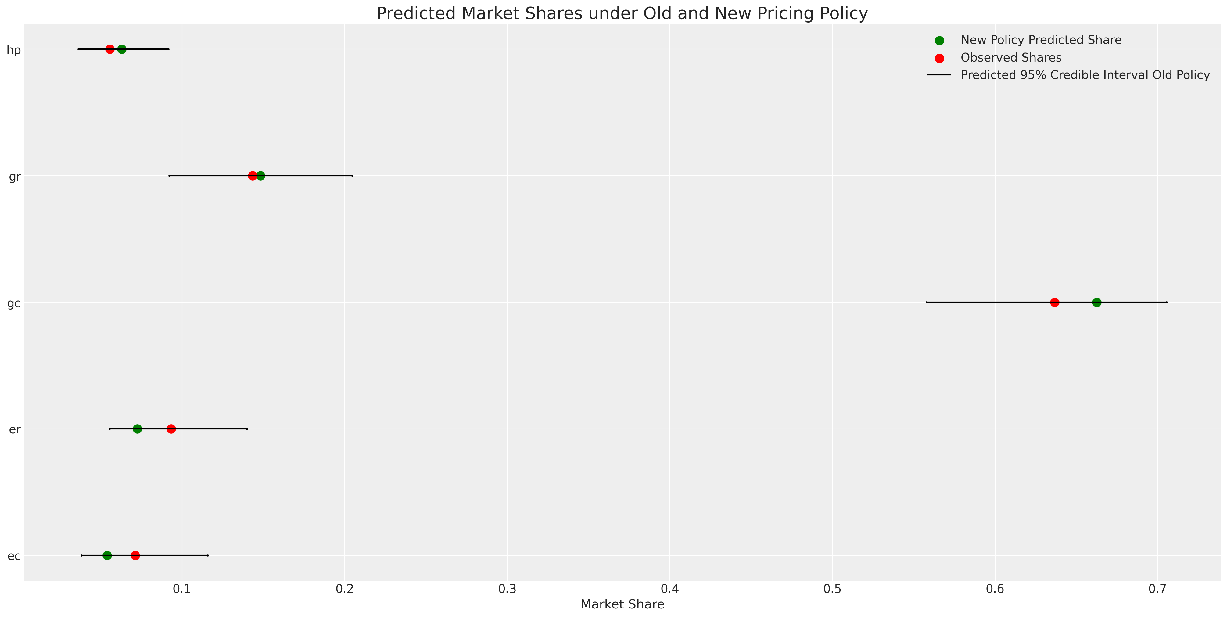
Counterfactual Shares

Counterfactual Reasoning

Interventions and Conditionalisation

• There is a sharp distinction between conditional probability distributions and probability under intervention
• In PyMC you can implement the do-operator to intervene on the graph that represents your data generating process.

Hierarchical Variations

Inducing covariance structures by allowing individual deviations from mean utilities.

Individual Heterogenous Utility

Repeated Choice and Hierarchical Structure

person_id	choice_id	chosen	nabisco_price	keebler_price
1	1	nabisco	3.40	2.00
1	2	nabisco	3.45	2.50
1	3	keebler	3.60	2.70
2	1	keebler	3.48	2.20
2	2	keebler	3.30	2.25

Individual Heterogenous Utility

\[ \begin{split} \begin{pmatrix} \color{red}{u_{i, nb}} \\ \color{purple}{u_{i, kb}} \\ \color{orange}{u_{i, sun}} \\ 0 \end{pmatrix} = \begin{pmatrix} (\color{red}{\alpha_{nb}} + \beta_{i}) + \color{blue}{\beta_{p}}p_{nb} + \color{green}{\beta_{disp}}d_{nb} \\ (\color{purple}{\alpha_{kb}} + \beta_{i}) + \color{blue}{\beta_{p}}p_{kb} + \color{green}{\beta_{disp}}d_{kb} \\ (\color{orange}{\alpha_{sun}} + \beta_{i}) + \color{blue}{\beta_{p}}p_{sun} + \color{green}{\beta_{disp}}d_{sun} \\ 0 + 0 + 0 \end{pmatrix} \end{split} \]

Individual Heterogenous Utility

In Code

with pm.Model(coords=coords) as model_4:
    beta_feat = pm.TruncatedNormal("beta_feat", 0, 1, upper=10, lower=0)
    beta_disp = pm.TruncatedNormal("beta_disp", 0, 1, upper=10, lower=0)
    ## Stronger Prior on Price to ensure 
    ## an increase in price negatively impacts utility
    beta_price = pm.TruncatedNormal("beta_price", 0, 1, upper=0, lower=-10)
    alphas = pm.Normal("alpha", 0, 1, dims="alts_intercepts")
    beta_individual = pm.Normal("beta_individual", 0, 0.05,
     dims=("individuals", "alts_intercepts"))

    u0 = (
        (alphas[0] + beta_individual[person_indx, 0])
        + beta_disp * c_df["disp.sunshine"]
        + beta_feat * c_df["feat.sunshine"]
        + beta_price * c_df["price.sunshine"]
    )
    u1 = (
        (alphas[1] + beta_individual[person_indx, 1])
        + beta_disp * c_df["disp.keebler"]
        + beta_feat * c_df["feat.keebler"]
        + beta_price * c_df["price.keebler"]
    )
    u2 = (
        (alphas[2] + beta_individual[person_indx, 2])
        + beta_disp * c_df["disp.nabisco"]
        + beta_feat * c_df["feat.nabisco"]
        + beta_price * c_df["price.nabisco"]
    )
    u3 = np.zeros(N)  # Outside Good
    s = pm.math.stack([u0, u1, u2, u3]).T
    # Reconstruct the total data

    ## Apply Softmax Transform
    p_ = pm.Deterministic("p", pm.math.softmax(s, axis=1), dims=("obs", "alts_probs"))

    ## Likelihood
    choice_obs = pm.Categorical("y_cat", p=p_, observed=observed, dims="obs")

Individual Heterogenous Utility

Recovered Posterior Predictive Distribution

Individual Heterogenous Utility

Individual Preference

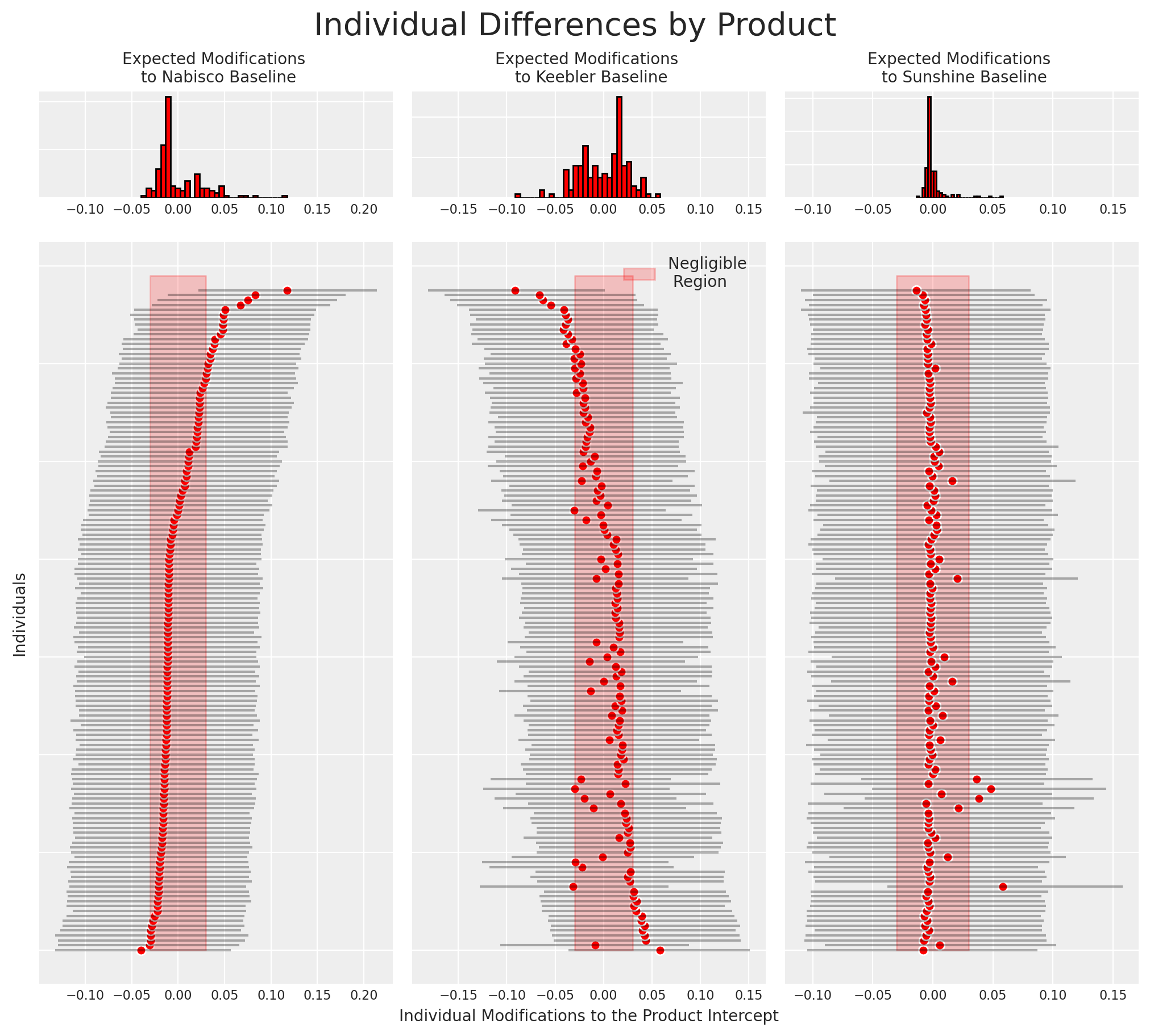
• Individual preferences can be derived from the model in this manner.
• The relationship between preferences over the product offering can be seen too

Conclusion

The World in the Model

We’ve seen a series of models, each one expanding on the last.

• Models should articulate the relevant structure of the world.
• They serve as microscopes. Simulation systems are tools to interrogate reality.
• Bayesian Conditionalisation calibrates the system against the observed facts.
• Bayesian Discrete choice models help us interrogate aspects of actors and their motivations under uncertainty.
• PyMC enables us to easily build and experiment with those models.
• Causal inference is plausible to degree that we can defend the structural assumptions. Bayesian models enforce tranparency and justification of structural commitments.

“Models… [are] like sonnets for the poet, [a] means to express accounts of life in exact, short form using languages that may easily abstract or analogise, and involve imaginative choices and even a certain degree of playfulness in expression” - Mary Morgan in The World in the Model